Guest post by Tamino
In a paper, “Heat Capacity, Time Constant, and Sensitivity of Earth’s Climate System” soon to be published in the Journal of Geophysical Research (and discussed briefly at RealClimate a few weeks back), Stephen Schwartz of Brookhaven National Laboratory estimates climate sensitivity using observed 20th-century data on ocean heat content and global surface temperature. He arrives at the estimate 1.1±0.5 deg C for a doubling of CO2 concentration (0.3 deg C for every 1 W/m^2 of climate forcing), a figure far lower than most estimates, which fall generally in the range 2 to 4.5 deg C for doubling CO2. This paper has been heralded by global-warming denialists as the death-knell for global warming theory (as most such papers are).
Schwartz’s results would imply two important things. First, that the impact of adding greenhouse gases to the atmosphere will be much smaller than most estimates; second, that almost all of the warming due to the greenhouse gases we’ve put in the atmosphere so far has already been felt, so there’s almost no warming “in the pipeline” due to greenhouse gases already in the air. Both ideas contradict the consensus view of climate scientists, and both ideas give global-warming skeptics a warm fuzzy feeling (but not too warm).
Despite the celebratory reaction from the denialist blogosphere (and U.S. Senator James Inhofe), this is not a “denialist” paper. Schwartz is a highly respected researcher (deservedly so) in atmospheric physics, mainly working on aerosols. He doesn’t pretend to smite global-warming theories with a single blow, he simply explores one way to estimate climate sensitivity and reports his results. He seems quite aware of many of the caveats inherent in his method, and invites further study, saying in the “conclusions” section:
Finally, as the present analysis rests on a simple single-compartment energy balance model, the question must inevitably arise whether the rather obdurate climate system might be amenable to determination of its key properties through empirical analysis based on such a simple model. In response to that question it might have to be said that it remains to be seen. In this context it is hoped that the present study might stimulate further work along these lines with more complex models.
What is Schwartz’s method? First, assume that the climate system can be effectively modeled as a zero-dimensional energy balance model. This would mean that there would be a single effective heat capacity for the climate system, and a single effective time constant for the system as well. Climate sensitivity will then be
S=τ/C
where S is the climate sensitivity, τ is the time constant, and C is the heat capacity. Simple!
To estimate those parameters, Schwartz uses observed climate data. He assumes that the time series of global temperature can effectively be modeled as a linear trend, plus a one-dimensional, first-order “autoregressive” or “Markov” or simply “AR(1)” process [an AR(1) process is a random process with some ‘memory’ of its previous value; subsequent values y_t are statistically dependent on the immediately preceding value y_(t-1) through an equation of the form y_t = ρ y_(t-1) + ε, where ρ is typically required to be between 0 and 1, and ε is a series of random values conforming to a normal distribution. The AR(1) model is a special case of a more general class of linear time series models known as “Autoregressive moving average” models].
In such as case, the autocorrelation of the global temperature time series (its correlation with a time-delayed copy of itself) can be analyzed to determine the time constant τ. He further assumes that ocean heat content represents the bulk of the heat absorbed by the planet due to climate forces, and that its changes are roughly proportional to the observed surface temperature change; the constant of proportionality gives the heat capacity. The conclusion is that the time constant of the planet is 5±1 years and its heat capacity is 16.7±7 W • yr / (dec C • m^2), so climate sensitivity is 5/16.7 = 0.3 deg C/(W/m^2).
One of the biggest problems with this method is that it assumes that the climate system has only one “time scale,” and that time scale determines its long-term, equilibrium response to changes in climate forcing. But the global heat budget has many components, which respond faster or slower to heat input: the atmosphere, land, upper ocean, deep ocean, and cryosphere all act with their own time scales. The atmosphere responds quickly, the land not quite so fast, the deep ocean and cryosphere very slowly. In fact, it’s because it takes so long for heat to penetrate deep into the ocean that most climate scientists believe we have not yet experienced all the warming due from the greenhouse gases we’ve already emitted [Hansen et al. 2005].
Schwartz’s analysis depends on assuming that the global temperature time series has a single time scale, and modelling it as a linear trend plus an AR(1) process. There’s a straightforward way to test at least the possibility that it obeys the stated assumption. If the linearly detrended temperature data really do behave like an AR(1) process, then the autocorrelation at lag Δt which we can call r(Δt), will be related to the time constant τ by the simple formula
r(Δt)= exp{-Δt/τ}.
In that case,
τ = – Δt / ln(r),
for any and all lags Δt. This is the formula used to estimate the time constant τ.
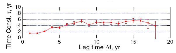
And what, you wonder, are the estimated values of the time constant from the temperature time series? Using annual average temperature anomaly from NASA GISS (one of the data sets Schwartz uses), after detrending by removing a linear fit, Schwartz arrives at his Figure 5g:
Using the monthly rather than annual averages gives Schwartz’s Figure 7:
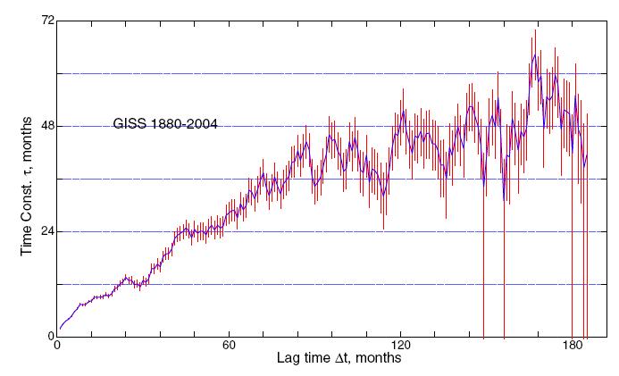
If the temperature follows the assumed model, then the estimated time constant should be the same for all lags, until the lag gets large enough that the probable error invalidates the result. But it’s clear from these figures that this is not the case. Rather, the estimated τ increases with increasing lag. Schwartz himself says:
As seen in Figure 5g, values of τ were found to increase with increasing lag time from about 2 years at lag time Δt = 1 yr, reaching an asymptotic value of about 5 years by about lag time Δt= 8 yr. As similar results were obtained with various subsets of the data (first and second halves of the time series; data for Northern and Southern Hemispheres, Figure 6) and for the de-seasonalized monthly data, Figure 7, this estimate of the time constant would appear to be robust.
If the time series of global temperature really did follow an AR(1) process, what would the graphs look like? We ran 5 simulations of an AR(1) process with a 5-year time scale, generating monthly data for 125 years, then estimated the time scale using Schwartz’s method. We also applied the method to GISTEMP monthly data (the results are slightly different from Schwartz’s because we used data through July 2007). Here’s how they compare:
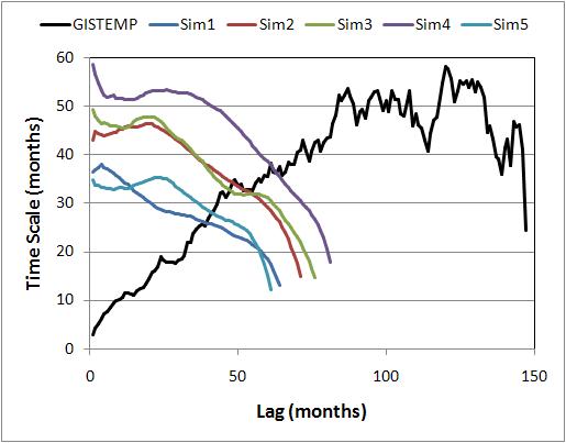
This makes it abundantly clear that if temperature did follow the stated assumption, it would not give the results reported by Schwartz. The conclusion is inescapable, that global temperature cannot be adequately modeled as a linear trend plus AR(1) process.
You probably also noticed that for the simulated AR(1) process, the estimated time scale is consistently less than the true value (which for the simulations, is known to be exactly 5 years, or 60 months), and that the estimate decreases as lag increases. This is because the usual estimate of autocorrelation coefficients is a biased estimate. The word “bias” is used in its statistical sense, that the expected result of the calculation is not the true value. As the lag gets higher, the impact of the bias increases and the estimated time scale decreases. When the time series is long and the time scale is short, the bias is negligible, but when the time scale is any significant fraction of the length of the time series, the bias can be quite large. In fact, both simulations and theoretical calculations demonstrate that for 125 years of a genuine AR(1) process, if the time scale were 30 years (not an unrealistic value for global climate), we would expect the estimate from autocorrelation values to be less than half the true value.
Earlier in the paper, the AR(1) assumption is justified by regressing each year’s average temperature anomaly against the previous year’s and studying the residuals from that fit:
Satisfaction of the assumption of a first-order Markov process was assessed by examination of the residuals of the lag-1 regression, which were found to exhibit no further significant autocorrelation.
The result for this test is graphed in his Figure 5f:
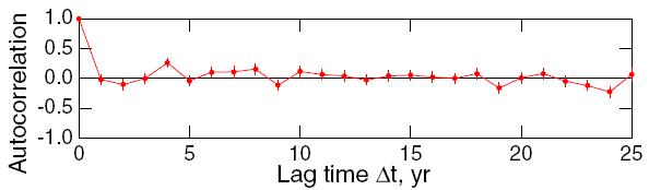
Alas, it seems this test was applied only to the annual averages. For that data, there are only 125 data points, so the uncertainty in an autocorrelation estimate is as big as ±0.2, much too large to reveal whatever autocorrelation might remain. Applying the test to the monthly data, the larger number of data points would have given this more precise result:
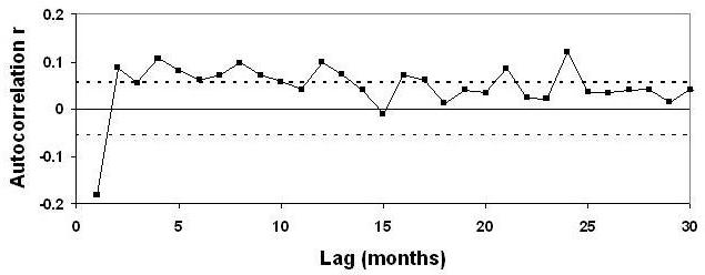
The very first value, at lag 1 month, is way outside the limit of “no further significant autocorrelation,” and in fact most of the low-lag values are outside the 95% confidence limits (indicated by the dashed lines).
In short, the global temperature time series clearly does not follow the model adopted in Schwartz’s analysis. It’s further clear that even if it did, the method is unable to diagnose the right time scale. Add to that the fact that assuming a single time scale for the global climate system contradicts what we know about the response time of the different components of the earth, and it adds up to only one conclusion: Schwartz’s estimate of climate sensitivity is unreliable. We see no evidence from this analysis to indicate that climate sensitivity is any different from the best estimates of sensible research, somewhere within the range of 2 to 4.5 deg C for a doubling of CO2.
A response to the paper, raising these (and other) issues, has already been submitted to the Journal of Geophysical Research, and another response (by a team in Switzerland) is in the works. It’s important to note that this is the way science works. An idea is proposed and explored, the results are reported, the methodology is probed and critiqued by others, and their results are reported; in the process, we hope to learn more about how the world really works.
That Schwartz’s result is heralded as the death-knell of global warming by denialist blogs and Sen. Inhofe, even before it has been officially published (let alone before the scientific community has responded) says more about the denialist movement than about the sensitivity of earth’s climate system. But, that’s how politics works.
I see if your a proponent your free to post anything but your not allowing me to rebut Mr. Chase.
RE: 240
Yes lets look at what both you and he said:
Mr. Chase, this is a distinction without difference. You say he is not stating that CO2 and aerosols cancel each other out, but rather that the process of burning fossil fuels and burning biomass both produce CO2 and aerosols which cancel each other out and that means that means what? The difference is? CO2 and aerosols are not cancelling each other out? No, then what was wrong with the statement. On to point two! Lets really look at what was said, namely that in the future it is likelyto shift towards dominance of CO2. The key word is likely. He does not say it ‘will’ happen, just that it ‘may’ happen. What does he say that actually happening is the non-CO2 GHGs are the source of 20th century warming.
I do not see what your third point has to do with what I posted. As of this point there is a theory that CO2 will cause temperature to rise but there has been none. Seems a pretty weak theory if CO2 has gone up 40 percent yet CO2 has caused no warming!
Then you make the unsupported statement:
“It is also worth noting that there has been a reduction in the production of aerosols as of 1970, and as such, the effects of carbon dioxide have been masked to a smaller degree since then.” What study do you have that contradicts Hansen in 2000? Please remember this is global not North America and Western Europe only.
Now you state:
But once again I refer to Hansen, who you are challenging who says that the IPCC is not looking at all forcings. Nothing you said all that you did nothing to address what Hansen said, which I have copied below again.
Next you state:
This is very disingenuous yet again. Tamino says that AR1 is not right. The IPCC says it is valid and you try and turn it around to be that I am saying that AR4 is wrong. Please point out where I said that? I believe that I said that the IPCC indicates that AR1 plus the linear trend is valid.
Next you state:
This is a weak attempt at misdirection. The fact is that the instrumented readings and the proxies do not match. The IPCC agrees with this. You are presenting opinion as to why they diverge without the facts to support your opinion.
Next you state:
Which is misleading since the warming is not happening on out side of the Antarctic Pen and there is still is mainly north of the Antarctic Circle. Please note I did not reference the Southern ocean, I reference the land which is cooling. The continent of Antarctica is cooling which does not match the GCM predictions.
You end with:
Yes, let them look at what I am saying. I have facts from studies while you have opinion without the facts to support them. You try to say that warming is by CO2 is not cancelled out by aerosols even though the process that produces man made CO2 produces the same aerosols which negate the CO2.
The fact is that Hansen says there has been no man made warming due to CO2. That it likely that there may be some in the future. If we quite producing CO2 by burning fossil fuels, the we also will stop the production of aerosols, and the net impact is none. If Tamino is right then the IPCC is wrong.
[Response: Vernon, we try to be flexible here, but you have repeatedly violated virtually every condition spelled out in our comments policy. Here, you continue to egregiously misrepresent the findings and views of James Hansen and it is hard to believe that the distortion is not intentional. We’ll post this, and allow other readers to comment on it, but this will be the last posting of yours that will go up until you choose to respect the ground rules. -mike]
I would first begin by saying that my comments about the lack of equillibrium do not preclude the AGW argument, and were not stated to disprove any theories. Thank you Jim (230) for expressing my point that as the system moves toward equillibrium it is continually disturbed and never achieves equillibrium, however, the statement, ““equilibrium” is a dynamic concept” is incorrect. Equillibrium has a specific meaning, and is in fact a black and white issue, either you have equillibrium or you don’t.
Hank (224), it would also seem that you agree with me. By stating,”The planet’s in radiative equilibrium when the temperature doesn’t change.” And then providing me with temperature reconstructions that show that temperature is always changing, are you not making my point?
Lastly, could someone please point out the error in the following statement:
The Stefan-Boltzmann law and constant apply only to black bodies.
The Earth is not a black body.
Therefore, the Stefan-Boltzmann law and constant do not apply to Earth.
Sure.
Natural “law” is not like human law.
Under human laws, either it applies to you or it doesn’t.
If you’re taxed, you’re taxed; if you’re not, you’re not.
Natural “law” is a statement of confidence level in an explanation, and an approximation.
Take black bodies. There aren’t any, in reality.
Does that mean the Stefan-Boltzmann law is like passing a law requiring payment of income taxes by fairies and elves?
No. It’s a reasonable description of what’s observed.
———–
Ok, your turn. Tell us where you are reading the things that you believe, so we can look at the source you consider reliable. You may have an old physics textbook, or a religious source, or have stumbled on one of the fossil fuel lobby’s public relations pages that pretends to be a science source, or be doing your own science. Without some source and comment about why you believe what you believe and where you’re getting the ideas you hold up here for comment, we don’t have much idea how to help you think independently about what you’re learning and do the math where needed.
There’s a 3rd response to the glass half empty/half full question. It’s “Aieeeee! The Alien has escaped!!”
(joke for the moderators. no need to post to the board.)
dhogaza, yeh, and all those things happening in the past few years because the global temperature went up a few hundredths of a degree??
Ellis, First, equilibrium is most definitely a dynamic concept in most physical systems–it simply means that the net change–averaged over suitable spatial, numerical and temporal scales–is negligible (note that I do not say zero). Do you contend that when a chemical system reaches equilibrium that there are no further chemical reactions? I would think not.
Second, there are ways of dealing with the fact that a body does not absorb/radiate as a true black body (e.g. emissivity), and modula these modifications, the same physics still applies. That is, Earth radiates (where it is quantum-mechanically able to) thermally, and in this portion of the spectrum the radiation looks roughly black body. There is a large body of work on these subjects. I recommend it to you.
dhogaza, to be fair, all those things might point to significant global warming. But the argument is not prima facie and, the point was, is mitigated somewhat with deterioration of other empirical data.
Vernon, your elementary ‘mistakes’ are easy to point out but it hasn’t helped. You have to be able to add and subtract and multiply and divide — basic arithmentic — at least, to understand the mistakes you’re making.
Take just one example (ignoring for now all the repeated misstatements you attribute to Hansen).
Consider this quote from you:
> You try to say that warming is by CO2 is not cancelled out
> by aerosols even though the process that produces man made
> CO2 produces the same aerosols which negate the CO2.
You’re failing subtraction:
(the Clean Air Act changed the ratio of sulfate to CO2 emitted from the then biggest polluters, coal power plants — the first half of the fossil fuels burned, up to about 1970, also produced lots of sulfates; the second half of the fossil fuels burned to date, since 1970, produced much less sulfate because it was scrubbed out;
You’re failing multiplication:
(sulfate added by burning coal falls out of the atmosphere in a few years; CO2 increases from burning coal stay higher for centuries because the chemical/biological processes that remove CO2 are overwhelmed by the rate of addition — so the ‘third half’ of the fossil fuels now being burned dirty in the Chinese and older US coal plants are again adding more sulfate, but all the earlier sulfate has fallen out already, while half of the earlier fossil CO2 is still in the atmosphere)
And you’re failing to check what you read.
Just ask, when you’re told something you like hearing (over at CA or wherever else): “how do you know that’s true, do you have a source?” — instead of grabbing that flag and rushing over here to wave it. Develop your skepticism. Please.
Vernon, allow me to introduce you to the concept of competing effects. When fossil fuel is burned, on the one hand we have CO2 emissions, which result in a positive forcing. On the other hand we have aerosols, which result in a negative forcing. These two forcings may initially be comensurate, and there may be no net observable warming or cooling. Should we then assume that they will always be equal and there will be no effect. The answer is not “no”, but rather “hell no”. CO2 persists for centuries in the atmosphere, while aerosols have a relatively short life. As long as new aerosols are streaming into the atmosphere you might not see a big effect, but aerosols have undesirable health and environmental effects. They are also technically easy to limit. Result, we will see fewer aerosols in the future. What happens now that aerosols are no longer there to mask the effect? CO2’s effects, formerly masked, now take off with a vengeance. You have to consider the temporal evolution of competing effects as well as their magnitude.
Thus, Hansen’s work should raise the level of concern for anyone who has understood it. Hint: That does not include you.
RE 258: Hank, please point to the study that shows the global aerosols have decreased since 1970.
You said:
Blockquote>You’re failing subtraction:
(the Clean Air Act changed the ratio of sulfate to CO2 emitted from the then biggest polluters, coal power plants — the first half of the fossil fuels burned, up to about 1970, also produced lots of sulfates; the second half of the fossil fuels burned to date, since 1970, produced much less sulfate because it was scrubbed out;
You make the assumption that environmental changes made in the North America and Western Europe are global. There may have been regional changes but Hansen did not indicate that what happened in 1970 had any impact in 2000. Since there has been no global warming from 2001-2006 per GISS, where is the CO2 based warming taking place?
You then went on to say:
Once again your presenting your opinion as fact. If what you say is so, then please present where Dr. Hansen was wrong in 2000? In the global context, aerosols and CO2 have been balanced for the last century. Now Dr. Hansen says that the process of burning fossil fuels and biomass produces both CO2 and aerosols and between them there is no impact on the climate’s temperature. That all current warming is due to other GHG’s.
As to where I get my information, I am willing to read what anyone says, but then I go and read the citations. If there are no citations, I ask for them, if they are not provided I do my own searches. I have noticed a trend to say anyone that is a skeptic must be a denier. I am sorry that I actually research what I present here, it must be confusing to have someone actually present facts and not opinions.
Re 252 Ellis: “Thank you Jim (230) for expressing my point that as the system moves toward equillibrium it is continually disturbed and never achieves equillibrium, however, the statement, ““equilibrium” is a dynamic concept” is incorrect. Equillibrium has a specific meaning, and is in fact a black and white issue, either you have equillibrium or you don’t.”
Sorry, I don’t see it as a black and white issue at all, rather that what constitutes equilibrium keeps changing as the system keeps being disturbed. I reiterate: equilibrium is not a static state.
Has or Is (all meanings of the word “is”) realclimate in any way (directly, indirectly, minorly, in theory, etc) funded by George Soros or his minions?
[Response: No, in all it’s meanings. – gavin]
Re #260: “Since there has been no global warming from 2001-2006 per GISS”
Someone ought to notify GISS to remove that suspiciously-upwards 2001-2006 trend from their global temperature graphs, e.g.:
http://data.giss.nasa.gov/gistemp/graphs/Fig.A2.lrg.gif
Vernon — With all due respect, I encourage you to carefully study
http://pubs.giss.nasa.gov/abstracts/2007/Hansen_etal_2.html
Vernon, there’s no point talking to you when you keep reposting this kind of claim, you’re just misreading Hansen’s work over and over.
You asked for help finding the sulfate info several previous times (remember you were searching for it, finding nothing, because you were misspelling it). The data is easy to find. Just another example:
http://www.tva.gov/environment/reports/envreports/04update/images/emissions.gif
Vernon, Por Deus! It’s not that hard to look this stuff up:
From Wikipedia
Examples of the atmospheric lifetime and GWP for several greenhouse gases include:
CO2 has a variable atmospheric lifetime, and cannot be specified precisely[18]. Recent work indicates that recovery from a large input of atmospheric CO2 from burning fossil fuels will result in an effective lifetime of tens of thousands of years.[19][20] Carbon dioxide is defined to have a GWP of 1 over all time periods.
http://en.wikipedia.org/wiki/Greenhouse_gas
And re: aerosol lifetimes:
“Unlike the long-lived greenhouse gases (GHGs), which are distributed uniformly over the globe, aerosol lifetimes are only a week or less [(2, 3), see Web table 1 for representative lifetimes of aerosols (1)], resulting in substantial spatial and temporal variations with peak concentrations near the source ”
http://www.sciencemag.org/cgi/content/full/294/5549/2119
As to the effect of the Clean Air Act on aerosols…well, what do you think it was intended to do? Note that Europe cleaned up its act about the same time, and the turning of Eastern Europe westward has resulted in incredible decreases in emissions of aerosols. Yes, China has increased its emissions, and that is having an effect, but the limited lifetime and localized source (compared to previously where the entire world was emitting this gunk) limits its effectiveness. So, while there is still an aerosol effect, the balance has shifted decidedly toward the warming effect of CO2. Competing effects, Vernon.
Oh, and maybe when you present your facts, you could try to spin them a little less. They seem pretty dizzy after you get done with them.
Ellis, equilibrium is defined over a span of time.
You’re defining it as forever, meaning it can’t ever happen.
Look at this page, and do a ‘find’ for the word ‘equilibrium’ — that may help you. The definition of the word in physics is not the definition you are insisting on.
http://www.pha.jhu.edu/dept/lecdemo/reese1.html
http://www.iop.org/EJ/abstract/0959-5309/50/3/308
Dear All,
This is interesting data, and the calculation of time constant vs. lag maybe particularly so.
The initial roughly linear relationship between the two might indicate that the mechanism involved is producing a constant phase delay for around the first ten years. This should not be a surprise as such a relationship is evident at short time-scales, i.e diurnal and seasonal. The delay of the response as a proportion of period being similar in both cases.
Surely the result found in this paper is not very surprising, in crude terms it just indicates that penetration (effective depth) increases with period. The longer the period the bigger the effective thermal capacity.
Systems that behave in such a way can always seem close to equilibrium and yet exhibit a very long tail.
Here we may have an example of everybody being correct. It is simply a matter of time-scales. Unfortunately if that is correct then the use of simple time constants to describe climatic response is simply inadequate.
Best Wishes
Alexander Harvey
RE # 260
Another opinion by Vernon
He said; [it must be confusing to have someone actually present facts and not opinions.]
And, he said
[Since there has been no global warming from 2001-2006 per GISS, where is the CO2 based warming taking place?]
I offer this quote from GISS:
[Global surface temperatures have increased about 0.6 degrees Celsius (1 degree Fahrenheit) since the mid-1970s. That increase culminated in 2005 with the highest surface temperatures ever recorded, according to a report released this month by James Hansen, director of NASA’s Goddard Institute for Space Studies, and colleagues.] at: http://tinyurl.com/2zt5qh
Vernon, give us some citations, not abbreviations. Please.
It’s always useful to refer to the IPCC, here’s the chart for sulfate worldwide over the past century. Note the change:
http://www.ccsm.ucar.edu/working_groups/Change/CCSM3_IPCC_AR4/images/20C3M_sulfate.gif
———–
Comparing the USA before 1970 with CHina now, not only has the background level of fossil CO2 changed, the latitude at which sulfates are emitted matters — photochemistry differs with latitude and amount of total sunlight:
“A commonality across future man-made emissions projections is a regional shift with decreases at NH midlatitudes and increases at the more photochemically active subtropical and tropical latitudes.”
http://www.pnas.org/cgi/content/full/103/12/4377
PNAS | March 21, 2006 | vol. 103 | no. 12 | 4377-4380
Cross influences of ozone and sulfate
precursor emissions changes on air quality and climate
Unger, Shindell, Koch, and Streets
Vernon,
Here is one paragraph (the first paragraph) in your recent response (#260) to Hank (#258)…
Vernon (#260) wrote:
Now let’s look at it sentence by sentence…
Vernon (#260) wrote:
Not evenly distributed, but global…
See:
Hemispheres
by Tamino at Open Mind
August 17th, 2007
http://tamino.wordpress.com/2007/08/17/hemispheres/
Vernon (#260) wrote:
Maybe not there, but according to his 2006 paper, the forcing due to carbon dioxide had exceeded that of tropospheric aerosol late in the twentieth century. Reflective aerosols at -1.0 w/m2 about 1974 (chart on pg. 22) and sulfates at -0.6 at about the same time (chart on pg. 24). Since then the influence of sulfates relative to carbon dioxide has been falling – same charts.
Climate simulations for 1880-2003 with GISS modelE
Hansen, et al
Clim. Dyn., doi:10.1007/s00382-007-0255-8, in press, 2007a.
http://pubs.giss.nasa.gov/docs/notyet/submitted_2006_Hansen_etal_2.pdf
I can get you the data as well if you want.
Vernon (#260) wrote:
Actually, per GISS, there has been warming – essentially the same upward trend as before – after the brief 1998 spike due to an exceptionally strong El Nino…
See the Image:
http://data.giss.nasa.gov/gistemp/graphs/USHCN.2005vs1999.lrg.gif
From the Webpage:
GISS Surface Temperature Analysis
Analysis Graphs and Plots
http://data.giss.nasa.gov/gistemp/graphs/
With the main text at:
GISS Surface Temperature Analysis
http://data.giss.nasa.gov/gistemp/
*
Incidentally, here is some material on the residence times of different aerosols…
Aerosol residence times…
3.3.2.1. Stratosphere
…
Large increases in H2SO4 mass in the stratosphere often occur in periods following volcanic eruptions (Trepte et al., 1993). Increased H2SO4 increases the number and size of stratospheric aerosol particles (Wilson et al., 1993).
3.3.2.2. Troposphere
…
The effect of aircraft sulfur emissions on aerosol in the upper troposphere and lower stratosphere is far larger than comparison of their amount with global sulfur sources suggests. The major surface sources of tropospheric sulfate aerosol include SO2 and dimethyl sulfide (DMS), both of which have tropospheric lifetimes of less than 1 week (Langner and Rodhe, 1991; Weisenstein et al., 1997).
Aviation and the Global Atmosphere
3.3. Regional and Global-Scale Impact of Aviation on Aerosols
3.3.2. Sulfate Aerosol
http://www.grida.no/climate/ipcc/aviation/036.htm
If a chunk of energy is put straight into the atmosphere, what happens to it?
Ray (248), I agree with the way your post is stated. Given the observations — a little ice melting here, some goofy bird migrations there, a few early cherry blossoms the past few years over there — we should wonder about them. More than that we should analyze them with some depth and dispatch and diligence, because they could portend some really bad stuff. But ironclad proof they ain’t, by a long shot, especially when some of the attending data gets muddled or tainted.
>little ice … goofy bird
Now that’s insensitivity in action. You blow off some of the earliest and longest time series observations made. They called it “Natural History”
http://cns.utexas.edu/communications/File/AnnRev_CCimpacts2006.pdf
http://www.cgd.ucar.edu/tss/aboutus/staff/bonan/ecoclim/index.htm
Hank (258) says, “Just ask, when you’re told something you like hearing (over at CA or wherever else): “how do you know that’s true, do you have a source?” — instead of grabbing that flag and rushing over here to wave it. Develop your skepticism. Please.”
Hank, I assume you are including direct quotes from Hansen in there, aren’t you?
Rod, exactly what data is getting muddled or tainted? Are there any data to suggest a cooling climate? ALL the data I know of suggest more energy going into the climate. So, as a physicist, I have to ask where that energy is coming from. To date there is only one candidate–anthropogenic CO2 emissions.
Now one can question how serious will be the effects of climate change. However, that requires modeling, and to date the models–and indeed the observational evidence–do not encourage optimism. You can question the validity of the modeling, but if the models don’t work, then we’re flying blind, and that is worse.
Think of it Rod–all the evidence points to warming AND to humans causing it. I just can’t understand how people can ignore ALL the evidence.
re Ray (259) Might as well hit on everyone. Actually, Ray I agree pretty much with your rebuttal to Vernon (though the deneanor leaves something to be desired, if you don’t mind me saying)… until your last sentence. This would be wildly humerous if it weren’t so serious: your response to someone quoting Hansen directly and verbatim is, “The emperor is dressed just fine! Just Fine!”
spilgard Says (263):
“Re #260: “Since there has been no global warming from 2001-2006 per GISS”
Someone ought to notify GISS to remove that suspiciously-upwards 2001-2006 trend from their global temperature graphs, e.g.:
http://data.giss.nasa.gov/gistemp/graphs/Fig.A2.lrg.gif”
On the other hand if you plot the 2001-2006 points from your rebuttal reference, you get little to no (average) temperature increase. Someone ought to notify GISS to remove that suspiciously-flat 2001-2006 average from their global temperature graphs.
[[The Stefan-Boltzmann law and constant apply only to black bodies.
The Earth is not a black body.
Therefore, the Stefan-Boltzmann law and constant do not apply to Earth.]]
Earth is not a black-body radiator, but it can be described by the Stefan-Boltzmann law if you include a term for emissivity, or better yet, if you break down the radiation into bands.
Vernon posts:
[[In the global context, aerosols and CO2 have been balanced for the last century.]]
Please cite a source and give the numbers involved. Aerosols dominated over CO2 from 1940 to 1970, causing a slight cooling; CO2 dominated over aerosols after that, causing warming. That’s my understanding. Where are you getting your numbers?
[[If a chunk of energy is put straight into the atmosphere, what happens to it?]]
Well, it probably depends on what type of energy you’re talking about, but if it’s generalized random energy, the most probably immediate effect is to heat the atmosphere locally.
Rod B observed:
“Given the observations — a little ice melting here, some goofy bird migrations there, a few early cherry blossoms the past few years over there — we should wonder about them. More than that we should analyze them with some depth and dispatch and diligence, because they could portend some really bad stuff.”
So your opinion is that all the observations only hint at global climate warming? Your position is not even at the level of confidence main stream science had twenty year ago. Do you consider the tens of thousands of man years of research on the subject during past years in different diciplines a futile effort?
“But ironclad proof they ain’t, by a long shot, especially when some of the attending data gets muddled or tainted.”
It would be interesting to know, which is an ironclad scientific proof for you. Could you elaborate more, give an example? Also, as Ray above inquired, what data specifically is muddled or tainted? Can you list some data sets you consider junk?
RE 277: Mr. Levenson
Hansen et al (2000) “Global warming in the twenty-first century: An alternative scenario” at Proceeding of the National Academy of Sciences August 15, 2000, 10.1073/pnas.170278997
To quote from Hansen in the report:
“Our estimates of global climate forcings indicate that it is the non-CO2 GHGs that have caused most observed global warming.”
Further, Hansen went on to say:
“Fossil fuel use is the main source of both CO2 and aerosols, with land conversion and biomass burning also contributing to both forcings. Although fossil fuels contribute to growth of some of the other GHGs, it follows that the net global climate forcing due to processes that produced CO2 in the past century probably is much less than 1.4 W/m2. ”
Further he repeats most of this in Hansen et al (2007) Climate simulations for 1880-2003 with GISS modelE. Clim. Dynam., in press, doi:10.1007/s00382-007-0255-8.
Why am I not being allowed to the posts that are directed at me?
RE: 271 Mr. Chase, lets look at what you said.
First let us go beyond the pictures and graphs and look at the actual numbers. GISSTEMP has the following global temps for 2001-2006 (J-D): 57, 69, 67, 60, 76, and 65. Please, where is the warming, can you point out where the warming is hidden in there? Which could also be why the big news was warming was going to start again after 2009. Do not get me wrong, I believe that we have had warming since the LIA. But I do not see accelerated warming that the instrumented direct readings are indicating. The proxies are not showing this accelerated warming.
Next take Hemispheres by Tamino at Open Mind August 17th, 2007. To quote the most often said phrase, where was it published and peer reviewed? Even for that matter, who is Tamino? What are his qualifications? I do not know so I can hardly accept him or his work as a basis for much of anything. Now much could be said about me, but I am not suggesting anything other than you read the published works.
Now as to Hansen’s 2006 work with ModelE let’s look at more than the pretty charts and pictures and see what Hansen actually had to say:
So Dr. Hansen says that the actual forcing is 1.9 Wm2 +/- 1.0 W/m2 which is pretty much the same thing found in his 2000 paper. It still comes out that Hansen believes that CO2 and aerosols cancel each other out.
But let’s assume that you are right and Dr. Hansen is wrong. The CO2 lasts a long time and the aerosols only a few months a best. The question remains, where is the warming due to CO2 if Hansen is wrong and aerosols are not countering them? We are still left with a 40 percent increase in CO2, which should mean that 70 percent of CO2 doubling’s impact should have happened, so where is it?
I see you pulled back from saying that IPCC was wrong about AR1. This brings us back to my starting point. There is no evidence of CO2 warming per Hansen in the 20th century so what is the evidence that climate sensitivity to CO2 is greater than what Dr. Schwartz suggests?
[Response: We’ve frequently discussed why you can’t use the 20th C alone as a constraint on sensitivity (aerosol uncertainty is too large). Thus the constraints come from combinations of different periods – the LGM, volcanic responses etc. ( https://www.realclimate.org/index.php/archives/2006/03/climate-sensitivity-plus-a-change/ ). For the 20th C, the only thing that matters is the net forcing and I discussed the attribution issue a while back (https://www.realclimate.org/index.php/archives/2006/10/attribution-of-20th-century-climate-change-to-cosub2sub/ ). – gavin]
> So your opinion is that all the observations only hint at global climate warming?
No, I was/am taking aim at the recent short-term anecdotal observations. It might also apply to other observations, but I’d have to think about that — and it would likely be “indicate”, not “hint”.
Look, there are nitwits on all spokes of the political wheel. If we are here to talk about science, look into what you read. Natural history began as anecdotes and observations, and people continue to observe the world and tell others what they see. You can do better than just dismissing any report you find inconvenient.
Re my #272 and the reply #278
Yes, the atmosphere will be heated locally, but then what happens?
I want to learn if any (what proportion) of this energy can escape into space, and if so, how?
We better find a way to quickly and efficiently remove carbon dioxide from the atmosphere.
Mother Nature takes a LONG time.
http://scientificamerican.com/article.cfm?chanID=sa003&articleID=000CC5E6-9AB7-153F-9AB783414B7F0000
We’re not talking centuries, we’re talking hundreds of thousands of years.
As long as the cost of emitting carbon is zero, we will continue to do so.
Energy prices have got to increase to reflect their true cost to the world.
This website has an interesting analysis (overly simplified at times though) of the problem and a possible solution: http://www.architecture2030.org/
>AEBAnner
Asked (repeatedly); answered (frequently)
e.g. https://www.realclimate.org/index.php/archives/2007/06/a-saturated-gassy-argument-part-ii/#comment-47031
Re #289
Thank you, but that’s a very long thread. Can you please be more specific. Is the matter dealt with in the initial essay, or in the following 600, or so, comments?
Jacob I (173) — Thanks for the link, which clarified the use of the approximate natural logarithm forcing for me.
Please check to see if I have it now:
Assume
C0 = 288 ppm (1850 CE carbon dioxide contentration)
C = 383 ppm (2007 CE carbon dioxide concentration)
then
RF = 5.35 ln(C/C0) W/m^2 = 1.485 W/m^2
which I suppose means that CO_2 radiative forcing now is 148.5% of what is was in 1880 CE?
So, Hank, you say Natural History has validated that anecdotal experiences put into inductive reasoning is valid scientific proof of the prognoses. Most scientists would not, with the exception of great amounts of anecdotal observations in a situation where that is all the evidence that can be mustered, could be considered a near or tentative (best we can do with what we have) proof. That, of course, becomes a judgement call — some say enough; others say we need more. And which of the disagreeing parties is the nitwit is also a judgement call.
Re: Myself 268,
I have found the time to have another look at the data and my suspicion that it says more about how the ocean cools itself than how the atmoshpere does so has increased.
The rising time constant is indicative of a thick body with internal heat transport mechanisms quite different to the simpler model presented. Thick bodies lose heat in the way indicated by the data unlike the model proposed.
Inspection of the data presented leads me to suspect that the time constants deduced are oceanic not atmospheric.
Best Wishes
Alexander Harvey
Um, I’m sure I didn’t mean or say that word salad.
I said read the science, don’t dismiss what you hear, look it up.
Hank, O.K.
I recommend Naomi Oreskes’ book chapter:
http://www.ametsoc.org/atmospolicy/documents/Chapter4.pdf
It’s about 35 pages, but formatted with a lot of white space.
The section, starting at page 80, on different models of science, falsification, consilience of evidence, etc is relevant to some of the discussions here.
David Benson posts:
[[C0 = 288 ppm (1850 CE carbon dioxide contentration)
C = 383 ppm (2007 CE carbon dioxide concentration)
then
RF = 5.35 ln(C/C0) W/m^2 = 1.485 W/m^2
which I suppose means that CO_2 radiative forcing now is 148.5% of what is was in 1880 CE?]]
You were doing all right until the last part. To contrast 2007 to 1850, feed in C = 383 for the first and C = 288 for the second. The forcing is 1.485 for the first case and 0.0 for the second case, not 1.0.
If anything the publicized reduction in arctic sea ice extent may UNDERstate the trend.
According to the Alfred Wegener Institute
http://www.awi.de/en/research/research_divisions/climate_science/sea_ice_physics/subjects/ice_thickness_measurements/
The ice is also thinning. Ice loss measurements based on extent only may be out by 50%.
Re: Myself 293,
The failure to find a single time constant reveals that the author’s model is far to simple for the task. The derivation of our climate’s sensitivity to forcing by this method is thereby flawed. That said the data should not be ignored. If the analysis is correct and the relationship between derived time constants and period is correct it could tell us something about how the oceans transport heat. The initial near linear relationship between time constants and period is indicative of an upper layer in which heat is transported by small scale mechanisms. The levelling off of the time constants with longer timescales could be indicative of the action of larger scale mechanisms at longer timescales.
Thick materials do not approach thermal equilibrium in an exponential fashion. Current temperatures contain a memory of prior temperatures on all time scales with different time constants, hence the observed increase of time constants with increasing periods. The leveling off at decadal periods might indicate that the memory is being wiped out by some mechanism that is removing heat and erasing the memory by mixing surface water with much deeper waters at these sort of timescales.
Best Wishes
Alexander Harvey
Barton Paul Levenson (297) — Thank you. I was misled by the term ‘Relative Forcing’. Should not this more acturately be termed ‘Additional Forcing’?
For example, in 1850 CE the forcing is X W/m^2, while in 2007 CE it is
X + 1.485 W/m^2.
Or do I still misunderstand?