Guest Commentary by Jim Bouldin (UC Davis)
How much additional carbon dioxide will be released to, or removed from, the atmosphere, by the oceans and the biosphere in response to global warming over the next century? That is an important question, and David Frank and his Swiss coworkers at WSL have just published an interesting new approach to answering it. They empirically estimate the distribution of gamma, the temperature-induced carbon dioxide feedback to the climate system, given the current state of the knowledge of reconstructed temperature, and carbon dioxide concentration, over the last millennium. It is a macro-scale approach to constraining this parameter; it does not attempt to refine our knowledge about carbon dioxide flux pathways, rates or mechanisms. Regardless of general approach or specific results, I like studies like this. They bring together results from actually or potentially disparate data inputs and methods, which can be hard to keep track of, into a systematic framework. By organizing, they help to clarify, and for that there is much to be said.
Gamma has units in ppmv per ºC. It is thus the inverse of climate sensitivity, where CO2 is the forcing and T is the response. Carbon dioxide can, of course, act as both a forcing and a (relatively slow) feedback; slow at least when compared to faster feedbacks like water vapor and cloud changes. Estimates of the traditional climate sensitivity, e.g. Charney et al., (1979) are thus not affected by the study. Estimates of more broadly defined sensitivities that include slower feedbacks, (e.g. Lunt et al. (2010), Pagani et al. (2010)), could be however.
Existing estimates of gamma come primarily from analyses of coupled climate-carbon cycle (C4) models (analyzed in Friedlingstein et al., 2006), and a small number of empirical studies. The latter are based on a limited set of assumptions regarding historic temperatures and appropriate methods, while the models display a wide range of sensitivities depending on assumptions inherent to each. Values of gamma are typically positive in these studies (i.e. increased T => increased CO2).
To estimate gamma, the authors use an experimental (“ensemble”) calibration approach, by analyzing the time courses of reconstructed Northern Hemisphere T estimates, and ice core CO2 levels, from 1050 to 1800, AD. This period represents a time when both high resolution T and CO2 estimates exist, and in which the confounding effects of other possible causes of CO2 fluxes are minimized, especially the massive anthropogenic input since 1800. That input could completely swamp the temperature signal; the authors’ choice is thus designed to maximize the likelihood of detecting the T signal on CO2. The T estimates are taken from the recalibration of nine proxy-based studies from the last decade, and the CO2 from 3 Antarctic ice cores. Northern Hemisphere T estimates are used because their proxy sample sizes (largely dendro-based) are far higher than in the Southern Hemisphere. However, the results are considered globally applicable, due to the very strong correlation between hemispheric and global T values in the instrumental record (their Figure S3, r = 0.96, HadCRUT basis), and also of ice core and global mean atmospheric CO2.
The authors systematically varied both the proxy T data sources and methodologicalvariables that influence gamma, and then examined the distribution of the nearly 230,000 resulting values. The varying data sources include the nine T reconstructions (Fig 1), while the varying methods include things like the statistical smoothing method, and the time intervals used to both calibrate the proxy T record against the instrumental record, and to estimate gamma.
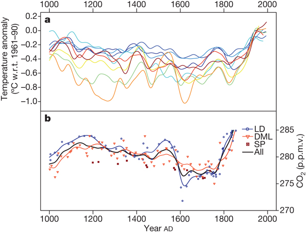
Figure 1. The nine temperature reconstructions (a), and 3 ice core CO2 records (b), used in the study.
Some other variables were fixed, most notably the calibration method relating the proxy and instrumental temperatures (via equalization of the mean and variance for each, over the chosen calibration interval). The authors note that this approach is not only among the mathematically simplest, but also among the best at retaining the full variance (Lee et al, 2008), and hence the amplitude, of the historic T record. This is important, given the inherent uncertainty in obtaining a T signal, even with the above-mentioned considerations regarding the analysis period chosen. They chose the time lag, ranging up to +/- 80 years, which maximized the correlation between T and CO2. This was to account for the inherent uncertainty in the time scale, and even the direction of causation, of the various physical processes involved. They also estimated the results that would be produced from 10 C4 models analyzed by Friedlingstein (2006), over the same range of temperatures (but shorter time periods).
So what did they find?
In the highlighted result of the work, the authors estimate the mean and median of gamma to be 10.2 and 7.7 ppm/ºC respectively, but, as indicated by the difference in the two, with a long tail to the right (Fig. 2). The previous empirical estimates, by contrast, come in much higher–about 40 ppm/degree. The choice of the proxy reconstruction used, and the target time period analyzed, had the largest effect on the estimates. The estimates from the ten C4 models, were higher on average; it is about twice as likely that the empirical estimates fall in the model estimates? lower quartile as in the upper. Still, six of the ten models evaluated produced results very close to the empirical estimates, and the models’ range of estimates does not exclude those from the empirical methods.
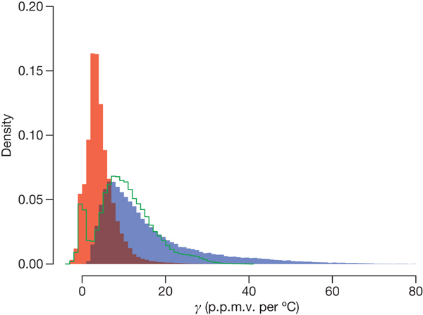
Figure 2. Distribution of gamma. Red values are from 1050-1550, blue from 1550-1800.
Are these results cause for optimism regarding the future? Well the problem with knowing the future, to flip the famous Niels Bohr quote, is that it involves prediction.
The question is hard to answer. Empirically oriented studies are inherently limited in applicability to the range of conditions they evaluate. As most of the source reconstructions used in the study show, there is no time period between 1050 and 1800, including the medieval times, which equals the global temperature state we are now in; most of it is not even close. We are in a no-analogue state with respect to mechanistic, global-scale understanding of the inter-relationship of the carbon cycle and temperature, at least for the last two or three million years. And no-analogue states are generally not a real comfortable place to be, either scientifically or societally.
Still, based on these low estimates of gamma, the authors suggest that surprises over the next century may be unlikely. The estimates are supported by the fact that more than half of the C4-based (model) results were quite close (within a couple of ppm) to the median values obtained from the empirical analysis, although the authors clearly state that the shorter time periods that the models were originally run over makes apples to apples comparisons with the empirical results tenuous. Still, this result may be evidence that the carbon cycle component of these models have, individually or collectively, captured the essential physics and biology needed to make them useful for predictions into the multi-decadal future. Also, some pre-1800, temperature independent CO2 fluxes could have contributed to the observed CO2 variation in the ice cores, which would tend to exaggerate the empirically-estimated values. The authors did attempt to control for the effects of land use change, but noted that modeled land use estimates going back 1000 years are inherently uncertain. Choosing the time lag that maximizes the T to CO2 correlation could also bias the estimates high.
On the other hand, arguments could also be made that the estimates are low. Figure 2 shows that the authors also performed their empirical analyses within two sub-intervals (1050-1550, and 1550-1800). Not only did the mean and variance differ significantly between the two (mean/s.d. of 4.3/3.5 versus 16.1/12.5 respectively), but the R squared values of the many regressions were generally much higher in the late period than in the early (their Figure S6). Given that the proxy sample size for all temperature reconstructions generally drops fairly drastically over the past millennium, especially before their 1550 dividing line, it seems at least reasonably plausible that the estimates from the later interval are more realistic. The long tail–the possibility of much higher values of gamma–also comes mainly from the later time interval, so values of gamma from say 20 to 60 ppm/ºC (e.g. Cox and Jones, 2008) certainly cannot be excluded.
But this wrangling over likely values may well be somewhat moot, given the real world situation. Even if the mean estimates as high as say 20 ppm/ºC are more realistic, this feedback rate still does not compare to the rate of increase in CO2 resulting from fossil fuel burning, which at recent rates would exceed that amount in between one and two decades.
I found some other results of this study interesting. One such involved the analysis of time lags. The authors found that in 98.5% of their regressions, CO2 lagged temperature. There will undoubtedly be those who interpret this as evidence that CO2 cannot be a driver of temperature, a common misinterpretation of the ice core record. Rather, these results from the past millennium support the usual interpretation of the ice core record over the later Pleistocene, in which CO2 acts as a feedback to temperature changes initiated by orbital forcings (see e.g. the recent paper by Ganopolski and Roche (2009)).
The study also points up the need, once again, to further constrain the carbon cycle budget. The fact that a pre-1800 time period had to be used to try to detect a signal indicates that this type of analysis is not likely to be sensitive enough to figure out how, or even if, gamma is changing in the future. The only way around that problem is via tighter constraints on the various pools and fluxes of the carbon cycle, especially those related to the terrestrial component. There is much work to be done there.
References
Charney, J.G., et al. Carbon Dioxide and Climate: A Scientific Assessment. National Academy of Sciences, Washington, DC (1979).
Cox, P. & Jones, C. Climate change – illuminating the modern dance of climate and CO2. Science 321, 1642-1644 (2008).
Frank, D. C. et al. Ensemble reconstruction constraints on the global carbon cycle sensitivity to climate. Nature 463, 527-530 (2010).
Friedlingstein, P. et al. Climate-carbon cycle feedback analysis: results from the (CMIP)-M-4 model intercomparison. J. Clim. 19, 3337-3353 (2006).
Ganopolski, A, and D. M. Roche, On the nature of lead-lag relationships during glacial-interglacial climate transitions. Quaternary Science Reviews, 28, 3361-3378 (2009).
Lee, T., Zwiers, F. & Tsao, M. Evaluation of proxy-based millennial reconstruction methods. Clim. Dyn. 31, 263-281 (2008).
Lunt, D.J., A.M. Haywood, G.A. Schmidt, U. Salzmann, P.J. Valdes, and H.J. Dowsett. Earth system sensitivity inferred from Pliocene modeling and data. Nature Geosci., 3, 60-64 (2010).
Pagani, M, Z. Liu, J. LaRiviere, and A.C.Ravelo. High Earth-system climate sensitivity determined from Pliocene carbon dioxide concentrations. Nature Geosci., 3, 27-30
#148–Edward, you are off-base. It was not me who made substantive statements without experimentation, but G & T. My point was simply that logic is sufficient (in many cases at least) to diagnose a misapplied analogy.
Perhaps your sermon on the philosophy of science could be redirected to them?
> That was why I asked if the expected date was 3010.
Want the month and day also? You’re asking for impossible precision.
Try this presentation (webex audio/slideshow), it’s good: http://ams.confex.com/ams/90annual/techprogram/paper_160915.htm
Jim, #146 (re #30):
Thanks, much! So my equations/graph are accurate.
As an aside, using natural or base 10 logs don’t really matter in the end (which is why I got to 1.41, too). It just changes the constant. Where a natural log gives you RF = 5.35*ln(C2/C1), a base 10 log gives you RF = 9.996*log(C2/C1), but you get exactly the same answer, so no worries there [the statement log(x)=ln(x)*(log(k)/ln(k) is true… sorry, my dad was a math professor, so I grew up liking that stuff].
[Response: OK, I figured it was along those lines, since you got the right value. The typo on the value of k threw me some.]
Yes, I agree completely on having to make a lot of (too many) assumptions, in particular whether or not any CO2 feedback has yet been realized, what the time scale is, and what the actual feedback values were in the models…. although what I’m computing (committed temperature) is mostly independent of time scale (we might see that temp in 20 years, or 200 years — the equation only says what we’ll reach, not when).
[Response: Right, but if part of what one is observing in the CO2 record is due to relatively fast feedbacks from T changes, say 10 years lag, your numerator includes that effect already. E.g. in 2010, at 388 ppm, let’s say of the difference of 108 from pre-industrial, 10 ppm is due to T induced feedback. That is, the numerator should be 378 + 10 = 388, therefore a 10ppm feedback, not a 0 ppm feedback. This will shift all your curves. Granted though, this only holds if the feedback is fast relative to the previous century’s T increase–jim]
The one exception is in determining feedback to date. But I’d be willing to bet (based on the mechanisms that would be involved) that we’ve seen negligible positive CO2 feedbacks to date, or we’ve nullified them with civilized behavior (forest clearing for wood products in place of forest fires), or perhaps there even would have been negative effects that we’ve also nullified the same way (e.g. increased plant growth and corresponding CO2 uptake has been restrained by annual harvesting and foresting of land).
[Response: Yes, I would tend to agree the feedback CO2’s probably not been great so far. But land use change has not offset it, but rather added to it, and in fact far oustrips it. One way to estimate gamma would be to use the info on time lags from the study, if we had it, and apply it to the industrial era. In fact that’s about the only way to estimate it, given the uncertainties in the carbon cycle’s fluxes–Jim]
But based on what I’ve read here since I did those computations, my takeaways are:
1) Time scales for CO2 feedback are probably longish. There could even be negative feedbacks in play right now (ocean uptake, increased plant growth) that will reverse and be replaced with longer term positive feedbacks (desertification/savanna-fication, etc.) that only arise when certain regional tipping points are reached (e.g. frequent and powerful droughts in the Amazon or central USA resulting in frequent and massive forest fires).
[Response:Hornet’s nest here. There definitely are strong negative feedbacks in play; the study is only trying to estimate the temperature induced feedback, not to quantify all feedbacks. There may well be “shortish” lag feedbacks that show up unexpectedly, especially if there are major droughts in forested areas. Your overall point is the most critical one though, and is exactly the critical point: temperature will drive many of these longer term feedbacks. Hence, gamma will likely be higher, at some point, than values given here–Jim]
2) The models are apparently not far from this study, so maybe I never should have plotted lines for overestimating feedback by 14 ppm/C or 21 ppm/C or 28 ppm/C. If the models are mostly in the 10 ppm/C range, and that’s where this study falls, then it doesn’t make sense to assume an “over estimation” much beyond 10 or 12 ppm/C (which would equate to zero or a possible slightly negative rather than positive feedback). It would be possible to go to any degree in the other direction, however (e.g. up to 30 ppm/C more CO2 feedback than modeled), but as I said already, that’s way too scary to even think about. It means we’re already committed to temperatures over 2C no matter what we do.
Anyway, I’ll take my bottom line result to be mostly accurate, then…
Each ppm/C more feedback than expected puts us one year closer to reaching the point of no return on hitting 2C, and puts the current temperature commitment 1/70 C higher.
Each ppm/C less feedback than expected puts us only one year further from reaching the point of no return on hitting 2C, and puts the current temperature commitment 1/70 C lower.
Which means that while this study is very interesting, the net impact of the unknowns on the climate (compared to anthro CO2) is marginal with respect to short term planning and timing. It only really matters if we’re so foolish as to let things get way out of control.
#95 on M-C:
You are right Jim and I am wrong, but we’re actually not far from semantics. When you repeatedly sample a parameter space to drive a model and accumulate a result distribution, that is statistical simulation. All we’re talking about is the sampling scheme. Exhaustively working through a discrete grid (as here) has the advantage of completely eliminating stochastic sampling bias, but at the expense of possible systematic bias (operator chooses the samples). It’s also very inefficient, as you point out. Am I saying this was a poor choice here? Of course not.
BTW, one cannot apply this approach without “a defined distribution” for each parameter. The authors chose those, although they don’t express it that way. For example, they made each of the temperature reconstructions and each of the CO2 series equally likely (discrete uniform distributions). They made similar choices for the smoothing splines and calibration intervals (continuous uniform distributions – which have defined bounds). Again, poor choices? Of course not. But choices; yes.
This is a powerful technique, but I don’t think one should pretend that it does things it does not. There’s just the faintest whiff of that in the author’s “…229,761 estimates for gamma” and, with respect, in your “full parametric experiment”. The results distribution necessarily depends on the parameter distributions. The degree of dependence here is not particularly high (as the supplementary demonstrates), which gives some confidence in the robustness of the result.
[Response: I guess I’m still not sure what it is exactly that you think is being pretended here. Nobody’s pretending that these are iron-clad results wrt the future–jim]
Much as I dislike schadenfreude, the news that climate denier Chris Monckton has come down with heat stroke is a delicious irony. No doubt he thinks it’s a case of frostbite.
Jim, re #153:
Yes, okay. Sounds right.
I think it’s interesting to consider that it’s probably a gross oversimplification (one of many, I know) to label gamma as a linear value. It’s quite probably not (e.g. 1 C may give you 10 ppm, but the next 1 C might give you 20 ppm more if it comes too quickly on the heals of the first 1 C increase).
I’m rather afraid that one of the factors that we can’t easily quantify is that CO2 is very much a part of the cycle of living things, and living things, given time, would adapt and compensate at least to some small degree. But if it happens too fast for ecosystems to adjust (e.g. for plants better adapted to the changed environment to assume a CO2 mitigating role) the effects could be far worse.
I don’t suppose anyone is doing a study to itemize and parametrize the various potential specific, individual CO2 feedbacks in the system. It would be interesting to see a time-line with all of the “coulds” and their dependencies (e.g. if precipitation falls below X and temperature above Y, which might be expected sometime between years A and B, then forest M could add between R ppm and S ppm CO2 to the atmosphere).
[Response: Oh yes. Lots going on there, from all angles. You just don’t hear much about it. I hope I can help change that.–Jim]
No one could ever put that into a single prediction of any sort (although they could all be built into models, and I assume many are), but it would be nice to sort of see what the list is, what’s big and small, what is surprising and unexpected, and what would add up… and, God forbid, check them off as they come to pass.
[Response: Wicked problem for sure. Constraining the carbon cycle budget is critical. We’re playing with fire with our ignorance of it. It’s the BIG wildcard.
152, Hank Roberts: Want the month and day also? You’re asking for impossible precision.
No, I am just asking for reasonable projections (and ranges of projections) for the next 25, 50, and 100 years. The figure that I first commented had no indication of when that much melting would have occurred.
Way O/T but was wondering if any here had heard of this project? Using peoples computers, laptops, etc for climate modeling (or Milky Way investigating or Malaria control, etc.)
http://climateprediction.net/content/about-climatepredictionnet-project
This could be a very economical way to help science and scientists!
151 Kevin McKinney: OK. Whoever. The point is that whoever is completely new to science needs to start with experiments. Science is something you DO, not something you READ. So, to whoever is completely new to science: The way you tell who is telling the truth and who is telling lies is by doing an experiment personally. For people with degrees in music or english or whatever that isn’t science, don’t be embarrassed to buy a chemistry [or other experiment] set from a toy store and start there. That is where the scientists started. Don’t worry about age.
You don’t need to know individually what all the forces are on a log rolling downhill are. You can roll the log down hill (or check the results of past log rolling downhill, measuring the grade) and check the velocity of the log through its rolling passage.
That you don’t know the energy loss through the uneven surface of the rough-hewn log doesn’t mean that gravity doesn’t pull down with a force of 9.8Newtons. That you measure that force as 10N +/- 1N from your log rolling measurements doesn’t mean that it’s outside that range because you didn’t account for a heavy clump of grass.
Yet dittos do exactly this for reconstructions of temperature sensitivity of CO2 changes.
EG: “Science is not so much a natural as a moral philosophy”
BPL: With the proviso that it’s a moral philosophy directed toward one particular end, finding the truth about nature. Being a scientist does not make you a moral person–witness Nobel prize winner Philip Lenard denouncing relativity as “Jewish Science,” Werner Heisenberg trying to build an A-bomb for Hitler, Bill Shockley on race and IQ, etc.
Miskolczi – is it all bunk or does he have a point? A piece on it would be great.
[Response: Bunk. – gavin]
#158 Leo G:
Yes, I use this screensaver but I have a 6 year old PC so I had to change the resource useage settings. This thing really sucks up resources while running in the background on default settings. :(
OT:
I just posted a new thread on my fledgeling blog titled: I am Saving 21% on my Electric Bill – So Can You!
I show my electric bill from Feb. 2008 vs. Feb. 2010 where I am now saving $39 per month because of a few green changes I made two years ago. I made my money back in less than six months.
If any of you have green stories to show savings please comment over there. Money talks louder than science apparently.
Re: 145. I think you need to consider uptake of CO2. The way I see the 10 ppm/C line is as an equilibrium state, which we are now well above due to injecting fossil carbon. When above this line there should be a net uptake, and when below a net CO2 emission. The uptake rate can be estimated from knowing we only see half the increase of CO2 that is injected, so it must be about 2 ppm/yr, given a rise of 2 ppm/yr. Whether the uptake rate is constant or in some way dependent on the distance from equilibrium is not easy to know, and also whether the 10 ppm/C line still applies in an increased carbon environment, but uptake is a first order term in this type of calculation that can’t be neglected.
Leo G says: 11 February 2010 at 11:57 PM
“Way O/T but was wondering if any here had heard of this project? Using peoples computers, laptops, etc for climate modeling (or Milky Way investigating or Malaria control, etc.)
http://climateprediction.net/content/about-climatepredictionnet-project”
Part of BOINC!
I have BOINC running here on an offsite backup server. The box uses a little more electricity as a result, ~430kWh/year for a cost of about $20. The “Al Gore is Fat” freaks will undoubtedly find it completely unacceptable, but on the other hand as long as the thing is installed on machines that otherwise would be running anyway I believe it’s a net benefit in terms of resources and of course it saves researchers a pile of cash.
BOINC allows you to choose your contribution from a smorgasbord of interesting projects.
> Septic Matthew says: 11 February 2010 at 10:03 PM
> I am just asking for reasonable projections (and ranges of projections)
Of what, for which location? I can help you a bit (a librarian could help you much more, if you go to a local library). You need to ask an answerable question.
Note the reply earlier, for sea level you need more than just a contour map. Exampple: http://www.epa.gov/climatechange/science/futureslc.html
> for the next 25, 50, and 100 years.
You’ve read the sections of the FAR and the recent followups on uncertainties in sea level rise? You’re aware of the range of uncertainty?
Here’s an example of the kind of information you can find if you look, for one particular area:
http://www.pacinst.org/reports/sea_level_rise/
Why not make the effort of looking for yourself, because you can specify the details important to you, and come back and comment on what you are able to find?
Sea level: see also:
http://www.nasa.gov/vision/earth/environment/sealevel_feature.html
Denialists aren’t playing Russian roulettte with the planet — see http://www.telegraph.co.uk/earth/environment/climatechange/7221110/Climate-change-sceptics-playing-Russian-roulettte-with-planet.html . It’s far worse than that, one bullet in a 6-chamber pistol. It’s more like they’re playing (let’s think of a word) SIBERIAN ROULETTTE, with 19 bullets in a 20-chamber pistol.
At least that’s what we can glean from the science, with the first studies reaching the .05 significance level in 1995, and the science becoming ever more robust since then.
(Note: take the extra “t” out of roulettte on the weblink — the spam filter wouldn’t let me post with the correct spelling)
167, Hank Roberts: You need to ask an answerable question.
I was responding to a post, and I asked a question to clarify the post. If someone suggests that there is possibly a 60m sea level rise, it is not unreasonable to ask that person when the sea level rise will occur.
Septic Matthew (157) — Three groups of engineers in three countries are all planning for 1+ meter SLR by 2100 CE.
171, David B. Benson: Three groups of engineers in three countries are all planning for 1+ meter SLR by 2100 CE.
I read that the Netherlands is planning for a 55cm – 110cm SLR. Is that one of the groups you know of, or is it a 4th group of engineers? Just curious.
Septic Matthew: engineers design for the top value in the range. Always. Then, then civil and structural engineers I know (out of an excess of caution) multiply by two. Or five. Or as much as they can get away with, really.
And what sort of building only stands for a hundred years? Many engineers have to take far longer timescales into account (which includes once in a century storms and similar considerations).
I’m curious: is your chosen nickname some kind of pun or in-joke?
> …Matthew
> 60m sea level rise
Who are you attributing this to?
It’s always important to cite your fact claims, even if you claim it’s something you read somewhere.
Then we can look at the source, instead of your questions, and check your recollection against a source.
Septic Matthew (172) & Didactylos (173) — The other two are in Britian and in California. While it is true that sea defenses have to take storm surge and so on into account, it seems the three groups all independently arrived at 1+ m as suitable with those in California, I think, actually having a somewhat larger figure.
While I suppose engineers in Venice are also alying plans, so far haven’t seen anythiing for New Orleans and around to Washington, D.C., where Foggy Bottom may well have to be renamed; SLR is not expected to be uniform due to mass redistribution and so changes in geodesy.
Septic Matthew & sea rise:
I actually asked the same Q about a 60 m rise some 2 years ago here, and the answers I got ranged from 2.5 m per century worst case to 5 meters per century worst case (based on paleoclimate research). Of course, we’re warming the world a lot faster, but still it takes a lot of time to melt ice, esp when winter still comes around each year to cool it down again. From these above rates, there could be a 60 m rise in 1,200 years or by 3,200. Or bec we’re warming up the world faster, maybe less than this.
MAPS: Here is a good set of maps with 100 m rise — you can click to get close-ups of coast lines by clicking it: http://resumbrae.com/archive/warming/100meter.html
I was especially interested bec I was writing a screenplay, HYSTERESIS, set in the future of a dying world, that had nevertheless managed to invent time travel, and sent a soldier back to kill the fictitious U.S. pres (so his better VP could take over tha steer the country/world on a path to avert such future destruction). For cinematic effect, I wanted shots of DC in a 60 m rise (you’d see the top of the Capitol buidling and the W Monument), and used that timeline to set my story. BTW (don’t want to spoil the ending) but the hero fails to kill the pres (a pacifist woman gets to him), with an intereting outcome.
Only problem now with my screenplay is that hysteresis isn’t the worst that can happen (100,000 years of extreme warming in which most of life on earth dies out, but then comes back slowly to eventually flourish again). According to Hansen the worst, which he says is likely if we burn all fossil fuels, including tar sands and oil shale, is the Venus syndrome, in which ALL life on earth dies out. See: http://www.columbia.edu/~jeh1/2008/AGUBjerknes_20081217.pdf
So anyway, if I rewrite my screenplay it will be under a different title: THE VENUS SYNDROME.
173, Didactylos: I’m curious: is your chosen nickname some kind of pun or in-joke?
Some kind, yes. On one of these threads I read the use of “septic” as a put-down pun on “sceptic”, so I self-agrandizingly took it as a name, like Yankees did with “yankee” and North Carolinians did with “tar-heel”, Indianans did with “hoosier”, and some others. And your name? I gather it means that you type with only two fingers, but you turn it into self promotion?
176, Lynn Vincentnathan: I actually asked the same Q about a 60 m rise some 2 years ago here, and the answers I got ranged from 2.5 m per century worst case to 5 meters per century worst case (based on paleoclimate research).
In most of the 20th century, the rate was 2mm/yr, but over the last 30 years might be higher at 3mm/yr.
174, Hank Roberts: Who are you attributing this to?
Take your own advice: check out post #107 by me.
Also, check out 63, by Hank Roberts. It’s a simple question, after all.
175, David Benson, thanks again.
155
Philip Machanick says:
11 February 2010 at 7:40 PM
“Much as I dislike schadenfreude, the news that climate denier Chris Monckton has come down with heat stroke is a delicious irony. No doubt he thinks it’s a case of frostbite.”
NO. You like schadenfreude. If you did not you would not have posted the above. Dont shroud your delight in falsity of presentation.
Monckton is in Australia (we are in summer here) after coming from your crappy Northern Hemisphere winter. This is not uncommon with visitors from the north.
162
John says:
12 February 2010 at 8:56 AM
“Miskolczi – is it all bunk or does he have a point? A piece on it would be great.
[Response: Bunk. – gavin]”
It has a point. AGW believers just hate it.
OT, but science is a cruel mistress> (xkcd for 2/12/10)
176
Lynn Vincentnathan says:
12 February 2010 at 7:46 PM
“Only problem now with my screenplay is that hysteresis isn’t the worst that can happen (100,000 years of extreme warming in which most of life on earth dies out, but then comes back slowly to eventually flourish again). According to Hansen the worst, which he says is likely if we burn all fossil fuels, including tar sands and oil shale, is the Venus syndrome, in which ALL life on earth dies out. See: http://www.columbia.edu/~jeh1/2008/AGUBjerknes_20081217.pdf”
Hansen’s hypothesis is nothing more than speculative crap with no empirical evidence. The earth cannot have a “Venus syndrome”.
Given that Jones has thrown Manns hockey stick under the bus and admited to the MWP and David Eyton, head of research and technology at British Petroleum who currrently fund, the CRU is investigating Jones; how much C02 would it take to re-inflate the tires on the bus, is the Earth was Venus and you all shared at least one brain?
[Response: Good question, I don’t know why we didn’t think of it–Jim]
RC: http://www.mediafire.com/?trm9gnmznde to which 181 Richard Steckis points does indeed have a 2.4 MB pdf attributed to Dr. Hansen that says we are in danger of going Venus [page 24] if we burn all of the coal and for sure go Venus if we burn all possible fossil fuel.
RC: Please please do a huge article on this possibility. Is it really Dr. Hansen’s work?
“The earth cannot have a “Venus syndrome”.
—-
Explain. Detail please.
RS: [Miskolczi] has a point. AGW believers just hate it.
BPL: If you think there is any scientific merit at all to Miskolczi’s jackass paper, you are a scientific illiterate.
#162 #179
A propos Miskolczi, and considering water vapour, any increase in (tropospheric) temperature (for whatever reason) will release water vapour (from cloud evaporation) leading to a further increase in temperature (GHG effect of water vapour). Since clouds are an inexhaustible supply of fresh water vapour this effect should cause catastrophic run away. It doesn’t. Why not?
“It has a point. AGW believers just hate it.”
It has two: AGW deniers just love it.
It has no science, but that’s not a problem for you, is it RS.
Steckis, have you even bothered to read the critiques that utterly demolish Miskolczi. The only possible merit I could find in it was the most “creative” application of the Virial Theorem–utterly wrong, but creative. I am almost afraid to ask this, Richard, but pray, what merit does this dog turd of a paper have other than as an exercise to Junior-level climate science students to find what’s wrong with it?
Hi,
I’d like to know if there’s a source where one can check global surface temperature on a daily basis.
Thanks a lot for your help and for your work.
[Westfield]– is it all bunk or does he have a point?
http://oddbooks.co.uk/oddbooks/westfield.html
Actually, there is a point and purpose to Miskolczi’s paper. Now, he and his family will be treated to lavish vacations in exchange for unintelligible presentations at conferences sponsored by right-wing think tanks (an oxymoron if there ever was one.)
Steckis:
Detailed blog science disproof of global warming in action …
Simon Abingdon, given your trolling tendencies, I’m reluctent to even engage. However, look up two things:
Claussius-Clapeyron equation
Convergent infinite series.
Andrew @182
Could you try that again in English or at least some other language comprehensible to humans?
RE: 184
Hey Garrett,
I concur, the eras around the Carboniferous M-P epochs may have been as close as the Earth would have come in the past; however, that was when Sol was cooler (On the order of 14/15ths…, (estimated), of the current incoming energy). Given the lesser heat content and high volume of water presence, there would not likely have been the initial conditions that existed on Venus.
It is likely a terrestrial or extra-terrestrial event may have covered a wide portion of the Earth in two separate planet wide events, eventually ending the Carboniferous era. (These events may have caused much of the die off of the Blue-Green Algae, that participated in the massive oxidation of iron and sulfur in the Earths land and oceans. In essence, high Carbon in the presence of high Oxygen content may have been enough to prevent the runaway heating during this time frame.) The resulting atmospheric chemistry was unlikely to support a Venus like climate.
The question is what would happen if you had high Carbon and higher Sulfates of dying biologic decay, without the high Oxygen content…, similar to what we are seeing in the oceans today?
Cheers!
Dave Cooke
simon abingdon — 13 February 2010 @ 5:58 AM postulates “…clouds are an inexhaustible supply of fresh water vapour…”
This postulate is refuted by observation; it was cloudy and 30F(-1C) last night here in North Carolina. Today, it is 33F(0.5C), not cloudy, and there is ~ 2in(5cm) of new snow on the ground. Clearly clouds are a finite(not “inexhaustible”) source of snow(not “water vapour”).
This thread about sea level rise of 10s of meters has been off-track for a while.
Septic Matthew should go to post # 92 (Susan Kraemer): “I realize that the year
3000 is outside the relevant policy time period, but as a matter of morbid interest
– what sea level is expected by 3000? What global average temperature? Have any
long term studies been done?” The question is clearly in reference to the year 3000.
Septic Matthew writes in # 107: “I thought that even a 20 foot sea level rise was only
a typo, and that there was no reliable forecast of anything like that much. Are we
talking here about the year 3010 or something?” So, yes we should be “talking here about
3010 or something” and not going back and forth needlessly.
Thanks for your valuable service RC!
190: Jiminmpls says:
http://oddbooks.co.uk/oddbooks/westfield.html
Thanks for that! Hilarious. The comments were the best part.
[Response: Something tells me I shouldn’t have started reading that…I already have a sideache–Jim]
Richard Steckis says: Miskolczi has apoint. AGW believers just hate it.
Ok. I’ll bite. What is the point? What are your qualifications for determining its veracity or do you just believe everything you read that purports to show that AGW can’t happen? I suspect the latter. Prove me wrong.
#177, Septic Matthew, & “In most of the 20th century, the rate was 2mm/yr, but over the last 30 years might be higher at 3mm/yr.”
Well, see, SM, this is where I’m sort of an expert. Have you ever had the duty of defrosting your SunFrost refrigerator (the one that save 90% electricity)? I thought so. It’s like this, the process starts out really slowly, then it starts speeding up, and toward the end it goes really fast. Furthermore, the paleoclimatologists have found that 2.5 m (some finding 5 m) per century (once the warming reaches a certain level, and the melting gets going in earnest) is what could happen….at least under the slow warming conditions of the past. Bets are sort of off for this unique, very fast, lickety-split warming we are involved with.
Here is one of the answers I got — the 5 m per century scenario:
—————————————————————
#181, Richard & “The earth cannot have a ‘Venus syndrome.'”
Now this is where we lay people diverge from the scientists — any scientist will tell you that we certainly will have a Venus syndrome (runaway warming) when the sun goes supernova.
Can it happen before that, is the question. According to Hansen (who really knows his science well), the sun is slowly but surely becoming brighter over the eons. IF you add that into consideration (and that during the earlier extreme CO2-warming scenarios the sun was less bright), AND you add in the fact that we are releasing CO2/CH4 into the atmosphere a lot faster than in past warming events, AND you consider that the slow negative feedbacks, such as weathering drawing down CO2, are happening too slow to make much difference, AND you consider that Jim Hansen is a nice guy who doesn’t understand just how evil human nature is (that there are enough people out there who would actually speed up their GHG emissions just to spite others, despite economic harm to themselves — enough of those types to make a real difference), then you can see that the situation looks fairly bleak.
(182)Comment by Andrew — 13 February 2010 @ 1:52 AM
For those of you who would like to know what Phil Jones actually said, you can read it here –
http://news.bbc.co.uk/1/hi/sci/tech/8511670.stm