There have been a number of studies which show that we can expect more extreme rainfall with a global warming (e.g. Donat et al., 2016). Hence, there is a need to increase our resilience to more rainfall in the future.
We can say something about how the rainfall statistics will be affected by a global warming, even when the weather itself is unpredictable beyond a few days.
Statistics is remarkably predictable for a large number of events where each of them is completely random (welcome to thermodynamics and quantum physics).
The normal distribution has often been used to describe the statistical character of daily temperature, but it is completely unsuitable for 24-hr precipitation. Instead, the gamma distribution has been a popular choice for describing rainfall.
I wonder, however, if there is an even better way to quantify rainfall statistics.
I have played around with the gamma distribution in an attempt to model daily rainfall statistics and its dependency on a set of physical factors. Without much success.
However, then I noticed that most daily rain gauge appeared to be almost exponentially distributed if I only included the rainy days (e.g. setting the threshold for a wet day at 1 mm).
When I plotted the histogram for rainfall on wet days with a log-y axis, I would mostly get a straight line of dots (see a typical example below).
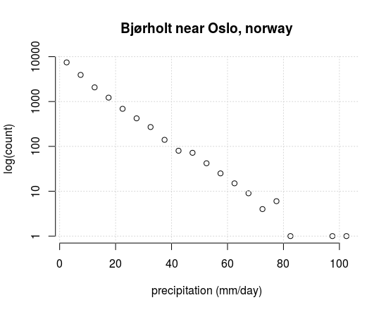
The nice thing with the exponential distribution (which is a particular case of the gamma function) is that it only requires one parameter to specify the mathematical curve: it’s the inverse of the mean value  .
.
I then used Bayes’ theorem to account for dry and wet days, where the probability for rainfall was taken to be the wet-day frequency  .
.
The advantage of this approach is that I now had two parameters which were easy to estimate: the wet-day mean precipitation (or mean rainfall intensity) and the wet-day frequency .
Furthermore, it turned out that is often closely connected to the wind direction, and can easily be predicted based on circulation patterns or sea-level pressure anomalies.
It was harder to find a systematic influence on , as it is likely affected by several factors, including the air moisture (which depends on temperature) and cloud top heights.
The total precipitation is the product of  , where
  is the number of days.
In other words, and tell me many things I needed to know about the rainfall statistics (there are other aspects too, such as the mean duration of dry/wet spells, the spatial extent, and whether it comes as rain, sleet, snow or hail).
The equation for estimating the probability for a rain event with amounts exceeding  can be written as (using 1-CDF for the exponential distribution):
(1) 
I have called it the “rain equation”, both because the name has not been taken and because it can provide many answers concerning rainfall.
It can address questions about the likelihood of heavy rainfall and whether it is due to an increase in the number of rainy days (e.g. due to changes in circulation) or because the rains have become more intense.
It is also on par with the normal distribution – in both cases, they are not meant to provide accurate probabilities for extreme events far out in the tails.
However, they are both capable of quantifying the probability of more moderate values, which can be illustrated in the figure below:
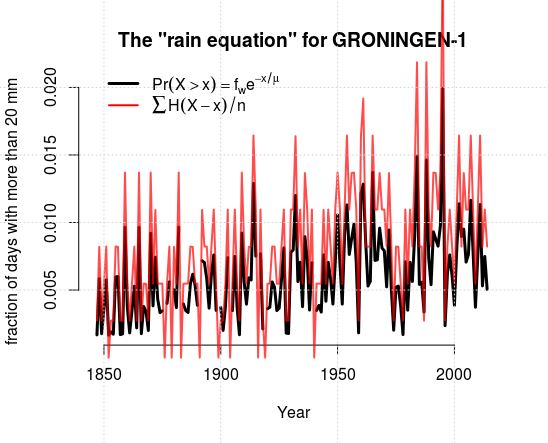
 refers to the Heaviside function, which is a mathematical way of expressing that I only counted the number of events with more than 30 mm/day each year in the observervations (the plot was made with the R-package
 esd and the command test.rainequation(loc='GRONINGEN-1',threshold=20)).The rain equation captures long-term changes as well as inter-annual variations. In this example, I used the annual wet-day mean precipitation and frequency estimated from the observations themselves to show its potential.
It can also be assessed against observations in a more systematic way, as in Figure 2:
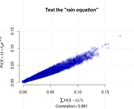
esd and the command scatterplot.rainequation()).A correlation of 0.98 is quite impressive, however, the rainfall is not perfectly exponentially distributed (Benestad et al., 2012). It nevertheless provides a means to address climate change connected to a change in either or .
We have used the rain equation in an attempt to downscale seasonal and decadal forecasts for precipitation (Benestad and Mezghani, 2015).
One thing that puzzles me, however, is that I cannot see this equation being used very much, despite the fact that it is so simple, seems so obvious, and can demonstrate impressive capabilities.
I would have thought it is an old formula. Perhaps one that has gotten out of fashion, but is documented in old papers that are not yet digitized and easy to google. Perhaps with a different name. Or have I missed something?
References
- M.G. Donat, A.L. Lowry, L.V. Alexander, P.A. O’Gorman, and N. Maher, "More extreme precipitation in the world’s dry and wet regions", Nature Climate Change, vol. 6, pp. 508-513, 2016. http://dx.doi.org/10.1038/nclimate2941
- R.E. Benestad, D. Nychka, and L.O. Mearns, "Spatially and temporally consistent prediction of heavy precipitation from mean values", Nature Climate Change, vol. 2, pp. 544-547, 2012. http://dx.doi.org/10.1038/nclimate1497
- R.E. Benestad, and A. Mezghani, "On downscaling probabilities for heavy 24-hour precipitation events at seasonal-to-decadal scales", Tellus A: Dynamic Meteorology and Oceanography, vol. 67, pp. 25954, 2015. http://dx.doi.org/10.3402/tellusa.v67.25954
Hi Rasmus,
I think exponential and mixed exponential distributions (the sum of multiple fitted exponential distributions) are fairly common in statistically modeling rain.
Here’s one with exponentials:
Richardson, C. W. (1981), Stochastic simulation of daily precipitation, temperature, and solar radiation, Water Resour. Res., 17(1), 182–190, doi:10.1029/WR017i001p00182.
One with mixed exponentials:
Foufoula-Georgiou, E., and D. P. Lettenmaier (1987), A Markov Renewal Model for rainfall occurrences, Water Resour. Res., 23(5), 875–884, doi:10.1029/WR023i005p00875.
And one that compares mixed exponential with gamma:
Wilks, D. S. (1998). Multisite generalization of a daily stochastic precipitation generation model. Journal of Hydrology, 210(1), 178-191, doi:10.1016/S0022-1694(98)00186-3.
Cheers,
Angie
Hello
You may be interested in a transient probabilistic model for describing simulated daily precipitation in a regional climate model. Jalbert, J., A.-C. Favre, C. Bélisle, J.-F. Angers and D. Paquin, 2015 : Canadian RCM projected transient changes to precipitation occurrence, intensity and return level over North America. Journal of climate. 28(17) 6920-6937 http://journals.ametsoc.org/doi/full/10.1175/JCLI-D-14-00360.1
Dominique
I’ve used a mixed exponential (or hyperexponential) distribution for modeling gridded daily precipitation amount, and also discussed how to fit the parameters:
NY Krakauer, SM Pradhanang, J Panthi, T Lakhankar, AK Jha (2015), Probabilistic precipitation estimation with a satellite product, Climate, 3(2): 329-348, doi: 10.3390/cli3020329
Hi, I am a student at the Institute for Climate Change and Adaptation University of Nairobi. Is the formula applicable to the El Nino/ La Nina phenomenon that has such a major impact on our weather systems in East Africa?
Dear Rosemary. I think the formula should be quite universal, but you can try and see. If you have data and use R, you can use the tools in https://github.com/metno/esd (see the wiki-page for more documentation). -rasmus
Mixed exponential models drop out of Maximum Entropy modeling, which is the basis of Jaynes views of statistical physics (e.g. compatibility with Bayes theorem). Here’s a blog post for Iowa rainfall, which generates a Bessel function from the proper integration of exponential decline functions:
http://theoilconundrum.blogspot.com/2012/02/rainfall-variability-solved.html
Have a book out later next year on Mathematical GeoEnergy via Wiley which will include many different statistical and deterministic models for earth sciences. BTW, Looking for technical reviewers on the final manuscript.
Rosemary asks:
“Hi, I am a student at the Institute for Climate Change and Adaptation University of Nairobi. Is the formula applicable to the El Nino/ La Nina phenomenon that has such a major impact on our weather systems in East Africa?”
The challenge in these studies is to determine which climate behaviors are stochastic and which are deterministic. As Rasmus has shown in the post, regional rainfall distributions are likely stochastic. In contrast, behaviors such as ocean tides are highly deterministic and very predictable.
So in considering something like the ENSO El Nino phenomena, one first has to realize that it arises from a single process relating to an unpredictable oscillating (sloshing) dipole in the equatorial Pacific thermocline. I would find it highly unlikely that this dipole would be caused by a random process, although many scientists would differ on this view.
The key to test whether ENSO is as deterministic as ocean tides is to actually input the forcing due to the lunisolar cycles, and see if it can reproduce the ENSO cycles adequately. Apparently no one has done this because the assumption has always been that the ENSO cycles are too chaotic. You can be the judge for yourself:
http://contextearth.com/2017/11/22/the-enso-forcing-potential-cheaper-faster-and-better/
As the great Walter Munk has pointed out, tidal forcing in ocean dynamics always has to be considered as a first-order mechanism.
This model will also be in the book on Mathematical GeoEnergy and I will be presenting at next month’s AGU in NOLA.
There is a new study on PETM hydrology (conservative analog)
https://www.youtube.com/watch?v=-oQsjWrix1U
More intense rainfall events, following more wildfires
means more mudslides and debris flows. That’s climate change too.
Sorry, mangled that pair of links that got merged.
See Frank Ackerman’s great new book: “Worst Case Economics: Extreme Events in Climate and Finance”
When I was at NASA/GSFC in 1986 I attended seminars given by the team that was developing the Tropical Rainfall Measuring Mission (TRMM). A number of the seminars were concerned with the statistics of rainfall, which impact the sampling error of the satellite’s instruments. At this point I can’t recall much, but a look at the papers published by the TRMM group (Dr Gerald North was the project leader at the time) might be of interest.