Site Google Custom Search

RealClimate logo

11 May 2008

What the IPCC models really say

Filed under: — gavin @ 9:23 PM - (Español) (English)

Over the last couple of months there has been much blog-viating about what the models used in the IPCC 4th Assessment Report (AR4) do and do not predict about natural variability in the presence of a long-term greenhouse gas related trend. Unfortunately, much of the discussion has been based on graphics, energy-balance models and descriptions of what the forced component is, rather than the full ensemble from the coupled models. That has lead to some rather excitable but ill-informed buzz about very short time scale tendencies. We have already discussed how short term analysis of the data can be misleading, and we have previously commented on the use of the uncertainty in the ensemble mean being confused with the envelope of possible trajectories (here). The actual model outputs have been available for a long time, and it is somewhat surprising that no-one has looked specifically at it given the attention the subject has garnered. So in this post we will examine directly what the individual model simulations actually show.


First, what does the spread of simulations look like? The following figure plots the global mean temperature anomaly for 55 individual realizations of the 20th Century and their continuation for the 21st Century following the SRES A1B scenario. For our purposes this scenario is close enough to the actual forcings over recent years for it to be a valid approximation to the simulations up to the present and probable future. The equal weighted ensemble mean is plotted on top. This isn't quite what IPCC plots (since they average over single model ensembles before averaging across models) but in this case the difference is minor.

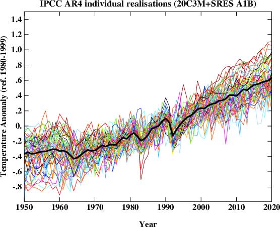
It should be clear from the above the plot that the long term trend (the global warming signal) is robust, but it is equally obvious that the short term behaviour of any individual realisation is not. This is the impact of the uncorrelated stochastic variability (weather!) in the models that is associated with interannual and interdecadal modes in the models - these can be associated with tropical Pacific variability or fluctuations in the ocean circulation for instance. Different models have different magnitudes of this variability that spans what can be inferred from the observations and in a more sophisticated analysis you would want to adjust for that. For this post however, it suffices to just use them 'as is'.

We can characterise the variability very easily by looking at the range of regressions (linear least squares) over various time segments and plotting the distribution. This figure shows the results for the period 2000 to 2007 and for 1995 to 2014 (inclusive) along with a Gaussian fit to the distributions. These two periods were chosen since they correspond with some previous analyses. The mean trend (and mode) in both cases is around 0.2ºC/decade (as has been widely discussed) and there is no significant difference between the trends over the two periods. There is of course a big difference in the standard deviation - which depends strongly on the length of the segment.

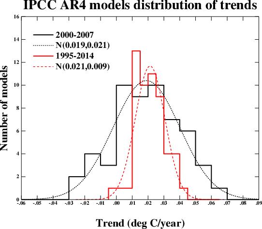
Over the short 8 year period, the regressions range from -0.23ºC/dec to 0.61ºC/dec. Note that this is over a period with no volcanoes, and so the variation is predominantly internal (some models have solar cycle variability included which will make a small difference). The model with the largest trend has a range of -0.21 to 0.61ºC/dec in 4 different realisations, confirming the role of internal variability. 9 simulations out of 55 have negative trends over the period.

Over the longer period, the distribution becomes tighter, and the range is reduced to -0.04 to 0.42ºC/dec. Note that even for a 20 year period, there is one realisation that has a negative trend. For that model, the 5 different realisations give a range of trends of -0.04 to 0.19ºC/dec.

Therefore:

  • Claims that GCMs project monotonic rises in temperature with increasing greenhouse gases are not valid. Natural variability does not disappear because there is a long term trend. The ensemble mean is monotonically increasing in the absence of large volcanoes, but this is the forced component of climate change, not a single realisation or anything that could happen in the real world.
  • Claims that a negative observed trend over the last 8 years would be inconsistent with the models cannot be supported. Similar claims that the IPCC projection of about 0.2ºC/dec over the next few decades would be falsified with such an observation are equally bogus.
  • Over a twenty year period, you would be on stronger ground in arguing that a negative trend would be outside the 95% confidence limits of the expected trend (the one model run in the above ensemble suggests that would only happen ~2% of the time).

A related question that comes up is how often we should expect a global mean temperature record to be broken. This too is a function of the natural variability (the smaller it is, the sooner you expect a new record). We can examine the individual model runs to look at the distribution. There is one wrinkle here though which relates to the uncertainty in the observations. For instance, while the GISTEMP series has 2005 being slightly warmer than 1998, that is not the case in the HadCRU data. So what we are really interested in is the waiting time to the next unambiguous record i.e. a record that is at least 0.1ºC warmer than the previous one (so that it would be clear in all observational datasets). That is obviously going to take a longer time.

This figure shows the cumulative distribution of waiting times for new records in the models starting from 1990 and going to 2030. The curves should be read as the percentage of new records that you would see if you waited X years. The two curves are for a new record of any size (black) and for an unambiguous record (> 0.1ºC above the previous, red). The main result is that 95% of the time, a new record will be seen within 8 years, but that for an unambiguous record, you need to wait for 18 years to have a similar confidence. As I mentioned above, this result is dependent on the magnitude of natural variability which varies over the different models. Thus the real world expectation would not be exactly what is seen here, but this is probably reasonably indicative.

We can also look at how the Keenlyside et al results compare to the natural variability in the standard (un-initiallised) simulations. In their experiments, the decadal mean of the period 2001-2010 and 2006-2015 are cooler than 1995-2004 (using the closest approximation to their results with only annual data). In the IPCC runs, this only happens in one simulation, and then only for the first decadal mean, not the second. This implies that there may be more going on than just the tapping into the internal variability in their model. We can specifically look at the same model in the un-initiallised runs. There, the differences between first decadal means spans the range 0.09 to 0.19ºC - significantly above zero. For the second period, the range is 0.16 to 0.32 ºC. One could speculate that there is actually a cooling that is implicit to their initialisation process itself. It would be instructive to try some similar 'perfect model' experiments (where you try and replicate another model run rather than the real world) to investigate this further though.

Finally, I would just like to emphasize that for many of these examples, claims have circulated about the spectrum of the IPCC model responses without anyone actually looking at what those responses are. Given that the archive of these models exists and is publicly available, there is no longer any excuse for this. Therefore, if you want to make a claim about the IPCC model results, download them first!

Much thanks to Sonya Miller for producing these means from the IPCC archive.

Update: Since some people have asked, the test for consistency (at 95% confidence) between the ranges seen in the models in figure 2 and real world trends is that the difference in means must be less than the twice the pooled standard deviation (and since the pooled s.d. is always larger than the s.d. in the models alone, it is trivially true that if the observed mean trend is within the 95% range of the models, it is consistent). See Lanzante 2005 for more info. All observational global SAT trends pass that test. Under no reasonable circumstances is an 8 year trend of -10 deg C/decade (that is 48 s.d. away from the mean) or even -1 deg C/decade going to be consistent with the models. For 7 year trends (beginning of 2001 to end of 2007), the model spread is approximately N(0.2,0.24) in deg C/dec - a little wider than the 8 year trends seen in the figure and there are 10 model simulations with negative trends.


462 Responses to “What the IPCC models really say”

  1. Donald E. Flood Says:

    So, to give one possibility, if the global mean temperature from 2050 to 2070 would end up being lower than the 1950 to 1970 global mean temperature, would that be enough to falsify the IPCC projections, assuming no volcanic eruptions, cometary impacts, etc.?

    [Response: …and that the trajectories of the GHGs and aerosols looked something like this scenario. Yes. - gavin]

  2. Richard Pauli Says:

    A caveat clearly seen on some IPCC charts:
    “Model-based range excluding future rapid dynamical changes in ice flow” Was this authored in 2005 or 2006?

    We cultivate confusion by failing to have constant IPCC studies and updated reports.

  3. A. Fucaloro Says:

    It would be impossible to deconvolve a trend signal caused by CO2 increase if the climate were mediated by a cycle that is long enough and strong enough. Do we know for sure that the medieval warming and subsequent Little Ice Age are not manifestations of such a cycle?

  4. tharanga Says:

    A relevant post; some sceptics love to say that the projections have been wrong, without actually knowing what the projections were.

    Some basic questions:

    If I understand it correctly, Keenlyside et al attempted to achieve more realistic realizations by using realistic initial values. Can you explain the standard ‘un-initiallised’ ensemble approach? Surely, a model that runs over time requires some sort of initial conditions; are these randomly chosen for each realization within the ensemble? It couldn’t be that random, though - to some extent, they must be constrained by observational data, no?

    Also, I’ve noticed that the various models tend to agree with each other within hindcasts, but there is rather more of a spread in the future projections. I’m told that the hindcasts are honest exercises, and not curve-fits, but in that case, shouldn’t there be more of a spread amongst the models in the hindcasts, as well?

    Finally - any attempts I’ve seen to judge prior model projections involve picking the results for the scenario (A1B, or what have you) which came closest to the actual forcings over the period in question. Instead of that, why not dig up those prior versions of the models and re-run them with the actual forcings: CO2, sulphates, volcanos, etc? It’s the range of unforced natural variability we are interested in here, not the ability of modelers to predict external forcings.

  5. One Salient Oversight Says:

    I love the “Pinatubo dip” in the first graph (1991).

    Maybe there is some legitimacy in the idea of “Dr Evil” to seed the upper atmosphere with particulates via 747s… but it only works in the short term. Once the aerosols dissipate, the curve keeps going up.

  6. David Says:

    When the models show cooling for a few years, is this due to heat actually leaving the (simulated) planet, or due to heat being stored in the ocean ?

    [Response: You’d need to look directly at the TOA net radiation. I would imagine it’s a bit of both. - gavin]

  7. Sascha Samadi Says:

    Thanks for the interesting and easy to understand read, Gavin. It’s hard for me to understand why some people apparently have a hard time distinguishing between individual model runs and ensemble means. It doesn’t seem to be too complicated…

  8. Gareth Evans Says:

    Back to scientific business and a welcome post by Real Climate. The important message in layman terms is that we must not confuse “weather” with climate. The greenhouse gases we emit warm the earth - this has been known for a long time (back to Arrhenius). The temperature of the earth would be much colder, roughly that of the moon, were it not for green house gas warming. Extra global energy, from increased greenhouse gas concentrations in the atmosphere, is redistributed around the earth by natural circluation processses. These are complex processses that may be interelated. In adition, there are natural cyclic events that may affect weather (and climate) and the unexpected (e.g. a significant volcanic erruption) is always a possibility. There will always be “weather” fluctuations and the various climate models produce a range of possible future outcomes. So, what we must focus on in this debate are the mean trends (and climate). This is exactly what IPCC and groups, like Real Climate, have been telling us. We need to develop ways, however, of introduing a regional focus into this debate and the important role of other warming influences such as land use, urbanisation etc. This would help to improve the general understanding and wider acceptance of the issues involved. The focus on global, annual means does not always make the necessary local impact (and may be concealing important subtleties - such as any seasonal impact variations of an increasing global temperature).

  9. pete best Says:

    So in the grand scheme of GCM analysis these recent model runs that made it into the media as cooling are what exactly, inadequate? I am desperately attempting to find out the reason why a reputable preliminary scientific analysis went to the media spouting this via a peer reviewed journal when in actual reality the analysis seems flawed.

    Is it statistics or the methods used I wonder. I just feel that the public are left frustrated and confused as to the reality of AGW. No wonder the deniers are still in the game when this sort of science is splattered all over the media large bold fonts.

  10. Klaus Flemløse Says:

    I will be pleased if you can answer the following question:

    Is the variation in the number of sunspots, the ENSO, changes in the thermohaline circulation and other periodic phenomenon included in the IPCC simulations? How good are then simulations to replicate the variations in the global temperature ?

    For me it is unlikely to see a monotonic increasing global temperature.

    [Response: Some of the models include solar cycle effects, all have their own ENSO-like behaviour (of varying quality) and THC variability. - gavin]

  11. Nylo Says:

    Certainly, weather influences climate trends.

    Is there ANY chance that the observed temperature increase since the 70s (and till 1998) is due mainly to weather (PDO, ENSO, cosmic rays, sun irradiation, solar cycles, cloud cover), or is weather only going to be responsible for cooling or a lack of warming?

    Is current La Niña “weather”? If so, was El Niño in 2002 and 2005 weather as well? Should we then say that the high temperatures we saw those years were because of weather, and not climate? Are their temperature records dismisable then? If not, will 2008’s decadal low temperature record be dismisable when it happens?

    I saw nobody claim anything about how weather influences the apparent climate trend when it was an all-rise problem in the nineties. But now that we are not warming, weather comes to rescue of the AGW theory.

    You have confidence in the models because the average of the ensemble seems to explain well the somewhat recent warming. But what if the warming was caused by weather? It is possible, because reality is just one realisation of a complex system. So all of your models could be completely wrong ans still their average be coincidental with the observations.

    In the GH theory, the surface temperatures increase because there is a previous increase of the temperature of the atmosphere, which then emits some extra infrared energy to the surface. In that scenario, the troposphere warms faster than the surface. Otherwise its emissions would not be too big and we would not have so much surface warming. This happens almost in every model run. There are only a handful of model runs that correctly guess nowadays mild tropospheric temperature increase in the tropics. I would like to know what is the surface temperature trend predicted by exactly those model runs which managed to get nowadays tropical tropospheric temperatures correctly. It seems like they got the “weather” right and seem more trustworthy, for me.

  12. bi -- Intl. J. Inact. Says:

    Nylo: cloud cover, solar activity, etc. has always been factored into climate models, from what I understand. And no climate model has been able to model the recent warming without taking CO2 into account.

    Gavin: Will you be discussing Monaghan et al.’s recent paper “Twentieth century Antarctic air temperature and snowfall simulations by IPCC climate models” (Geophy. Res. Lett.) some time? The handling of model uncertainties in the paper seems a bit weird to me…

    – bi, Intl. J. Inact.

  13. Olee Says:

    I would like to paraphrase the late Douglas Adams on this – to remind of us all of the “Whole Sort Of General Mish Mash” (WSOGMM) that one must consider in complex systems.

    Two model runs for a century starting from the exact same initial conditions but with the same forcing may well end up in different states (yielding different trends) at some point of the run. Different models with same or different initial conditions but same forcing also spread in their states throughout the runs. Hence there is a lot of WSOGMM going on as seen in Figure 1.

    What is rarely discussed is that WSOGMM is not something that is exclusively associated with climate models. WGSOGMM is an inherent property of the “real” climate system as well. It is most likely that if we had measurements of our instrumental period in one or several parallel universe ‘Earths’ the inter-annual to decadal temperature evolution of these parallel worlds would deviate from each other to some extent. The current near-decadal relaxation of the global temperature-trend may for example have started in 1994 or 2003 rather than 1998 on one of our ‘parallel planets’ since it is largely defined by the 1998 El Nino event – that may have occurred during any year when “conditions were favourable” on some particular ‘parallel universe’ Earth. Thus, to use our instrumental records as the “perfect answer” is probably faulty below some decadal time-scale because this notion mean we think that the climate system is 100% deterministic on this time-scale. This is, however, unlikely since many of the sub-decadal patterns (NAO, PDO, ENSO for example) seems to be resonating more or less stochastically.
    All this remind us that a relaxation of the temperature trend for a decade or so is not falsification of the multi-ensemble IPCC-runs - also because the real-world data represent only one realisation of the WSOGMM on these short time-scales.

  14. Barton Paul Levenson Says:

    Nylo posts:

    was El Niño in 2002 and 2005 weather as well?

    Were those, in fact, El Niño years? I knew 1998 was but I hadn’t heard about the other two. Does anybody know?

  15. Ray Ladbury Says:

    Nylo: Fascinating theory. Explain to me exactly how weather will cause warming over, say, 20 years. I will leave as an exercise to the reader a comparison of the amount of energy needed to warm Earth’s climate by 0.2 degrees and that of a hurricane. Here’s a hint. One’s gonna be a whole helluva lot bigger than the other.

  16. Nylo Says:

    I agree with #13, a relaxation of the temperature trend for a decade or so is not falsification of the multi-ensemble IPCC runs. In fact, a relaxation for 20 years would not be either. The problem with the models is that their error bars are so huge, compared to the trend that they are intended to predict, that they basically cannot be falsified during the academic lifetime of their creators, no matter what happens. However science MUST be falsifiable and at the same time not falsified by events in order to be science. As long as anyone claims that another 10 years of no warming or even cooling would not falsify the models, I cannot give the models any real value or contribution to science. A nice hobbie, at most.

    @12: That no climate model has been able to predict the recent warming without an increasing CO2 doesn’t mean that it is not possible, it only means that they all share common beliefs that could be right or could be not. For example, no climate model has been able to get right, at the same time, the current surface temperature trend and the current tropical tropospheric temperature trend, but still it is happening, they are roughly the same. Only non-GH influenced warming has such a fingerprint. How can they all be wrong?

    And then there is the fact that the models include things such as cloud cover. Given how unknown the process of cloud formation is, and given that their average results fail to correctly show the real anual variation of cloud cover - they all give too much cloud cover for winter and too little for the summer compared to reality, which means that the clouds of the models fail to cool as much as they cool in real life -, well, it doesn’t speak wonders of the models.

    Anyway, it looks interesting for me that the models cannot predict the warming without CO2, but on the other hand, they can predict cooling in spite of CO2 (so that falisification is imposible). How can it be? The models in Gavin’s article show a variability of up to 0.2ºC in a period of 20 years, but they cannot explain a 0.3ºC rise in global temperatures between 1980 and 2000 without CO2? Using a similar reasoning, I would admit as good a model which showed that only an increase of 0.1ºC between 1980 and 2000 was because of CO2, with the remaining 0.2ºC being weather. Such a model would predict immediate cooling now, and only a total +0.4ºC between now and 2100. And you could not say that such a model was falsified by the data either.

    [Response: You are too focussed on the global mean temperature. There are plenty of other trends and correlations that can be deduced from the models which can be independently validated (water vapour, sea ice, response to volcanoes/ENSO, ocean heat content, hindcasts etc.). Or you can go back twenty years and see what was said then. Either way, it is a balance of evidence argument. On one hand you have physically consistent models that match multiple lines of evidence, or … nothing. Given that the first indicates serious consequences for the coming decades, and the latter implies you have no clue, there is a big procrastination penalty for sticking your head in the sand. None of the issues you raise are ignored in the models and yet no model agrees with your conclusion. If there was, don’t you think we’d have heard about it? PS. you don’t need climate models to know we have a problem. - gavin]

  17. Nylo Says:

    @Ray Ladbury: it can. Gavin just showed it to you. The same model with just 5 runs can give differences of 0.2ºC in its trend for a period of 20 years. What is it, if not weather?

  18. Nylo Says:

    @ Barton Paul Levenson:

    ttp://www.cpc.ncep.noaa.gov/products/analysis_monitoring/ensostuff/ensoyears.shtml

  19. steven mosher Says:

    great post Gavin, that cleared up a lot of questons. thx.

  20. Ray Ladbury Says:

    Nylo, variability is not just weather–it includes initial conditions, and depending on the model may include variations in a variety of factors (many of which we could measure if they were occuring). Ultimately, what matters are long-term trends. Organisms are adapted to survive weather. Human civilization has done well to adapt to weather. However, sustained changes in climate are something that we haven’t had to deal with in about 10000 years, and certainly not on this order.
    To explain the trends of the past 20 years would take a veritable conspiracy of natural variations–or you could assume that a process that is known to operate is still operating. Me, I’ll stick with physics over conspiracy.

  21. steven mosher Says:

    re 17. well put Ray. It could be numeric drift, but I’m sure that is well accounted for. Gavin?

  22. Nylo Says:

    Gavin,

    One of the dangers of using an ensemble of models is that it can give you the false feeling that you cover every posibility. I will explain. The PDO is included in the models, as well as solar forcing, ENSO, etc. But because they are considered unpredictable, they are set random and averaged out by the ensemble of models because of pure statistics. They are actually ignored. And that is OK if you want to predict climate without weather, but then you cannot look at the real data and validate your climate-only models with it. Because real data is climate PLUS weather. So both temperature trends being similar says little until you use such a long period of time as to be able to claim that the weather component is irrelevant.

    In normal conditions, one century could be enough. But we are not in normal conditions. Why? Because of all the warming during the century, roughly a 50% of it has happened in only 20 years and is therefore possibly weather-influenced. If it is, we should start to see cooling anytime now, as I think we will. So only some of the remaining warming of the century can be trusted as climate change, and therefore it is not clear what you can compare your models to, in order to verify if their predictions can be trusted or not.

    What you cannot do is to say that the stable temperatures we have now are because of weather, and some hypothetical future cooling would be weather too, but the warming of the last decades of the 20th century was on the other hand “weather-clean”.

  23. Richard Treadgold Says:

    I’m surprised how many people take computer climate model forecasts over 50 years seriously when we still don’t get accurate predictions of the weather two weeks in advance. Uncertainty in projected temperature from models can approach ±55° after 50 years. Which is a forecast worth nothing.

    This is according to Patrick Frank at Skeptic Magazine, http://tinyurl.com/635bf8. I’m not without skill, but I’m no scientist, so I judge who sounds honest.

    [Response: Try judging who sounds credible. Frank’s estimate is naive beyond belief - how can it possibly be that the uncertainty is that large when you look at the stability of the control runs or the spread in the different models as shown above? - gavin]

    I’m more interested in the real world and the real climate. So, rather than asking what models tell us about variability, I’d like to ask about the science. What are the ramifications for the AGW hypothesis of the lack of atmospheric warming over the ten years since 1998? Arguably, since 1998 was driven by an exceptional El Nino, there’s been no real warming since about 1979, just going by eyeball. It’s up and down, but no trend you could hang your hat on. Temperature today is the same as 1979. See Junk Science.

    [Response: You are joking right? Junk Science indeed. - gavin]

    I can understand people shouting warnings about future warming, since models fire them up (hmmm, sorry about the pun, it was actually unintentional), but some people have been screaming about the world growing hotter right now. I honestly can’t see high temperatures anywhere.

    Last point: If CO2 is to warm the atmosphere, and warmer still with more CO2, then if CO2 rises but temperature is constant or falls, the theory is disproved. Done. Where is the faulty reasoning? Or what is the change to the theory?

    [Response: The ‘theory’ that there is no weather and no other forcings and no interannual and no interdecal variability would indeed have been falsified. Congratulations. Maybe you’d care to point me to any publications that promote that theory though because I certainly don’t recognise that as a credible position. Perhaps you’d like to read the IPCC report to see what theories are in fact being proposed so that you can work on understanding them. - gavin]

    Richard Treadgold

  24. Roger A. Pielke Sr. Says:

    Gavin - Your plot of the individual realizations is quite useful. To add to its value, I recommend that you also plot the global averaged upper ocean heat storage changes for each year in Joules that each model produces along with the resultant diagnosed global average radiative forcing in Watts per meter squared such as performed by Jim Hansen [see http://climatesci.colorado.edu/publications/pdf/1116592Hansen.pdf].

    [Response: Great idea - why don’t you do it? - gavin]

  25. Ray Ladbury Says:

    Has anybody else noticed how fixated the denialosphere is on Karl Popper? Everything is about “falsifiability”. It is as if the past 70 years of philosophy of science did not happen for them. Popper’s concept of falsifiability is important, but it isn’t particularly helpful when considering a complicated model with many interacting factors. The reason is that most of the factors included in the model probably contribute to some extent and especially for dynamical models, the selection of various ranges of parameters may be dictated (supported) by independent data. To “falsify” the model would mean giving up the explanatory and predictive power of a model where many aspects are right. Rather, it makes a lot more sense to keep the basic structure of a model with a proven track record and add additional factors as needed and supported by evidence. Alternatively, you could modify the strengths of various contributors–again as supported by evidence.

    It makes a lot more sense to look at this in terms of model selection (or even model averaging) than it does “falsification”. So all you denialists have to do is come up with a model that does a better job explaining the preponderance of information (and more) explianed by the current crop of GCM. Go ahead. We’ll wait.

    (crickets chirping)

  26. Michael Lucking Says:

    With these models, I assume the total heat absorbed by the yearly melting of ice has been included?

  27. Gaelan Clark Says:

    #21, Yeah Roger, why don’t you do it? I mean it’s not like Gavin won’t share his code with you, is it? Surely Gavin will give to you his complete model runs and the exact parameters that were included in all of them so that you can expand on his Science.
    He says it is a “Great idea”, so I expect you to have this information before you ask for it.

    [Response: Don’t be an ass. The data is all available at PCMDI and Roger has frequently expressed interest in it. I do think it is a good idea, but I have other things I am working on. The whole point of this post is to point people to the fact that the data is available and people should look at it for anything they particularly care about. If Roger cares about that metric, he should download it and look. I have not done so, and do not have the time to service every request that comes my way. FYI our complete model source code and runs are all available on the GISS web site. -gavin]

  28. dhogaza Says:

    I saw nobody claim anything about how weather influences the apparent climate trend when it was an all-rise problem in the nineties.

    Climate science predictss nothing about your willingness to pay attention, and the fact that you didn’t notice all the hoo-raw about the exceptionally strong El Niño in 1998 doesn’t mean that millions of other people didn’t.

  29. Alexander Harvey Says:

    Gavin,

    It is my understanding that once the all the known forcings are taken into account using their measured values the models reproduce the temperature history from 1950-present with a high degree of accuracy. Both in trend and in accounting for variation due to volcanoes. What they cannot easily account for is the precise timing of effects like ENSO.

    Viewing the difference between the mean of multiple runs (or similar process) and the real temperature record as the “weather” or the erractic component I believe that its amplitude is less than +/- .15C for around 90% of the time and peaks at around +/- 0.25C.

    Now visually your first figure is telling the same story which is heartening. If it was predicting a tighter band it would be contrary to reality.

    Is there a recognised “profile” of the erractic part of the real temperature record, i.e. how much of the time the record should be 0.1C, 0.2C, 0.3C etc above and below trend? I mean after all known forcings including volcanoes etc are taken into account.

    Your second figure seems to tell the same story. All the regression lines are confined inside a “pencil” of uncertainty with a width of about +/- 0.25C. The longer the pencil length you choose the tighter the degree C/decade band.

    It is possible that this may be the fundamental limit to the acuracy of prediction but in the long run 50 years plus (a very long pencil) it gives a very narrow band for the degree C/decade figure.

    Now what interests me is why the uncertainties for a doubling of C02 (or equivalent) are still so poorly constrained in comparison. (I think 3C +/- 1.5C is still the quoted band).

    We now have some reasonably good figures for what the oceans have done of the last 50 years and the amount of heat taken up by the oceans does constrain the value of the climatic sensitivity for the past 50 years. Is it the case that the models are making different assumptions about how the sensitivity will evolve in the coming decades or is it simply that the models are improved by constraining their runs during the known historic period and they then diverge in the future due to the lack of constraint? That is does the “pencil” turn into a “cone”. I can see no convincing tendency towards divergence in your first figure. Perhaps a figure extending a few more decades would help.

    Finally do the individual runs, that make up your first figure, simply reflect different initial conditions are certain parameters varied between runs.

    Best Wishes

    Alexander Harvey

    [Response: The variations for single models are related to the initial conditions. The variations across different models are related to both initial conditions and structural uncertainties (different parameterisations, solvers, resolution etc.). The two sorts of variation overlap. - gavin]

  30. Hank Roberts Says:

    http://julesandjames.blogspot.com/2008/05/are-you-avin-laff.html#comments

  31. Nylo Says:

    http://www.elsideron.com/GlobalTempPredictions.jpg

    In the graph of the link above you can see GISS temperature data for the last 125 years. On top of it, I have drawn one light blue line which would be approximately like the catastrophic predictions of the models (the trend being 1.5ºC/century in the end part, so not even as catastrophic as some of the models predict). Also on top of it, I have drawn a green line with an alternative forecast which would trust that the warming between 1980-2000 was mostly, but not all, due to weather. This line shows only a 0.6ºC/century warming, and would also NOT be falsified by real temperature data.

    As you can easily see, because of the last decade of stabilised temperatures, we are now at a crucial point. In dotted lines, again in blue and green, I have tried to represent what would be the logical evolution of temperature in order to more or less match each of the predictions. The 0.6ºC/century prediction desperately needs cooling ASAP, and I would call it falsified if it doesn’t cool within 2 years. But the 1.5ºC/century AGW prediction also needs some warming pretty quickly too or it would be about impossible to catch up with the prediction. I wouldn’t wait more than 5 years before deciding which of the 2, if any, is more accurate. I don’t think that stable temperatures with no warming or cooling would support any of the 2 predictions. It would rather prove both of them wrong.

    By the way, I chose a straight green line on purpose. The CO2 we emit is increasing, but on the other hand, the GH effect of any extra CO2 we emit is decreasing exponentially.

    [Response: No it’s not. The forcing is increasing slightly faster than linearly. - gavin]

  32. Patrick M. Says:

    re 26 (gavin):

    Could you post a link to where the source code can be downloaded?

    Thanks!

    [Response: The ModelE source code can be downloaded from http://www.giss.nasa.gov/tools/modelE or ftp://ftp.giss.nasa.gov/pub/modelE/ , the output data are available at http://data.giss.nasa.gov and the full AR4 diagnostics from all the models at http://www-pcmdi.llnl.gov/ipcc/about_ipcc.php - gavin]

  33. Ice Says:

    Thanks for this very interesting post.

    i was just wondering how independant, and then, not redundant, all these different climate models really were, that is, if one should not somehow account, when “averaging” them, for some particular -maybe historical - “closeness” between some of them (for example, i would think there aren’t 20-something different and independant schemes of sub-grid parametrization for convection, or cloudiness - are there? or maybe i’m raising a false problem here…)

    [Response: No, it’s a real issue. IPCC does exactly that. I didn’t bother. - gavin]

  34. Nylo Says:

    Gavin, the forcing by CO2 is measured in ºC for a DOUBLING, which means that it follows an exponentially decreasing trend: when we add 280 ppm we will have doubled, but in order to experience again the same achieved warming we would have to add a further 560 ppm, not a further 280. The more CO2 we already have, the more quickly we need to continue adding CO2 to mantain the same warming. It’s how the physics works. What really counts is how we change the existing concentration of CO2, the percentage of the change, not how much “raw” CO2 we add. Adding 5 ppm was quite more important when the concentration was 180 ppm than now.

    [Response: We all know that the forcing is not linear in concentration. But it isn’t decreasing, it is increasing logarithmically. And it is certainly not decreasing exponentially. - gavin]

  35. jae Says:

    Just squinting at those individual realizations, I sure don’t see any that show a ten-year long increase, level, or decreasing temperature.

    [Response: The histogram shows at least one that has a negative trend from 1995 to 2014, and there are nine that have negative trends from 2000 to 2007. For 1998 to 2007 there are 7 downward trending realisations (down to -0.15 degC/dec). Actual calculation trumps eyeballing almost every single time. - gavin]

  36. Bryan S Says:

    Re #20: Ray, It requires an anomalous accumulation of heat of about 0.2 W/M2 over a single annual period (maybe 18 months) to heat the atmosphere 0.3-0.4 degrees C. This compares to a modeled net upward radiative flux from the ocean surface of abound 0.7 W/M2 during the 1998 El Nino alone. Now consider that the observed change in upper ocean heat storage (net TOA radiative imbalance) that was observed over this same time interval, as reported in Willis 2004, is around +1.2 W/M2. This means that even though there was a theoretical loss of 0.5 W/M2 from the atmosphere to space as a result of the El Nino, the ocean still accumulated significant heat during the El Nino. So clearly weather processes exchange plenty of heat back and forth between the ocean, atmosphere, and space to accomplish considerable warming or cooling of the atmosphere over an annual to multi-decadal period. The real science question concerns whether this annual to multi-decadal intrinsic variability averages to a 0 trend over the period in question. My point is that there is no physical law that suggests that the inherent trend must in fact be 0. The notion is based on the ensemble mean of different GCMs run with stable CO2, all having similar core physics and slightly different parameterizations of weather processes. There is only one individual realization of the actual climate system however, and clearly, unforced variability can have a trend across many different scales. Roger Pielke Sr. has made an excellent point however, in stating that there is really no such thing as “natural variability”. It is kind of like making a white cake batter, and stirring in a little chocolate, and then trying to make a white cake and a chocolate cake from the same batter. Once the chocolate has been stirred in, you have a chocolate cake. The human influence including aerosols, landuse, and GHGs have already been stirred up together with natural variability.

    Gavin makes an important statement when he points out that many people have mistaken the range of model trajectories with uncertainty in the ensemble mean from multiple models. An important question to ask is why there is uncertainty in the ensemble mean, and is this uncertainty braketed properly (highside or lowside)? Another way to ask this is what are the variables controlling the uncertainty in the magnitude of the forced component of climate change. I suggest that as more physical processes are added to the models, that the range of uncertaintly will grow. Ice sheet dynamics included in the models might increase the highside, and more realistic representation of cloud feedback might increase the range on the lowside. Better landuse representation might go either way.

  37. Ray Ladbury Says:

    Nylo says: “The CO2 we emit is increasing, but on the other hand, the GH effect of any extra CO2 we emit is decreasing exponentially.”

    OK, I don’t have to go any further than this. How can you expect to be taken seriously when you haven’t even bothered to acquaint yourself with the physics of the model you are arguing against?

  38. Gary Plyler Says:

    Can you please explain why you have decided to base your bet on surface temperatures (Hadcrut) instead of satellite measurements of global atmosphere temperature? After all, no matter what corrections are made to account for urban heat island effect or for sensor relocation, they are corrections that cannot be independently verified. I really think that your bet should be based on sattelites that look at all the atmosphere with no local bias possible.

    [Response: The data and time periods for this wager are based purely on the targets suggested by Keenlyside et al. You will however find that no source of data is unaffected by structural uncertainty. - gavin]

  39. Axel Says:

    Gavin, great post. The discussion regarding the Keenlyside et al paper naturally has been focusing on what the paper is predicting. I’d be interested to hear comments about the fact that the paper claims to have made advances in multi-decadal climate prediction (title). Their figure 1d shows considerable improvement in skill (correlations) over the unintialized simulations over ocean areas. I understand that there is a similar paper (Smith et al.) that also shows that it is apparently possible to nudge models into reproducing decadal variability of the “real world” realization and use this for decadal climate prediction? Is this an appropriate reading? But maybe this is a discussion for a separate thread.

    [Response: We’ll discuss the K et al studies in greater depth at some point soon. - gavin]

  40. tamino Says:

    Re: #34 (Nylo)

    Gavin, the forcing by CO2 is measured in ºC for a DOUBLING, which means that it follows an exponentially decreasing trend: when we add 280 ppm we will have doubled, but in order to experience again the same achieved warming we would have to add a further 560 ppm, not a further 280. The more CO2 we already have, the more quickly we need to continue adding CO2 to mantain the same warming. It’s how the physics works.

    [sarcasm]Gavin is only a professional climate scientist — so he must not have known this.[/sarcasm]

    And by the way, CO2 isn’t increasing linearly, so it turns out that in the real world CO2 forcing is increasing faster than logarithmic, in fact over the time span of the Mauna Loa record it’s faster than linear.

  41. Ray Ladbury Says:

    BryanS., What is typically going on is a change in the amount of cold water that comes to the surface. However, what you are failing to consider is the fact that such changes do not persist for long. And if you have warming due to such a fluctuation in the absence of increased GHG, you get more radiation escaping to space (and vice versa). It is only with a ghg mechanism or a sustained trend in some other forcer that you get sustained warming. What is your candidate for a mystery sustained forcer?

  42. Gary Fletcher Says:

    We could have 10 consecutive years of .04 C global annual mean temp rise,
    each year being an “ambiguous” record, resulting in a cumulative .4 mean temp rise over the period, yet never have an “unambiguous” .1 C temp record year. Unless, of course, we keep a separate record of “unambiguous” years, so that unambiguous record years are considered separately from ambiguous ones. Which did you mean?

    [Response: After 3 years the previous record would have been unambiguously broken. - gavin]

    The GISS, in their 2007 summary, indicates that “projection of near-term global temperature trends with reasonably high confidence” can be made. They predict a record global temperature year “clearly exceeding that of 2005 can be expected within the next 2-3 years.” They base that prediction largely on the solar cycle. Your considerations are more general, even so, your graph indicates about a 2/3 chance of a record year in any three year period. Do you agree with the more confident and specific GISS prediction?

    http://data.giss.nasa.gov/gistemp/2007/

    [Response: The 50% level (ie. when you would expect to see a new record half the time) is between 1 and 6 years depending on how ambiguous you want to be. So it isn’t contradictory, but they are probably a tad more confident than these statistics would imply. - gavin]

  43. Mick Says:

    So what results would falsify this chart?

    Is it possible to observe something that contradicts the IPCC?

    [edit]

    [Response: Sure. Data that falls unambiguously outside it. - gavin]

  44. Lamont Says:

    I was playing around over the weekend with ENSO data and NASA global temperature data. I get a fairly good fit if I smooth the global temperature data to a 6 month average, advance the ENSO data by 6 months and divide by 10 (so a +1.0 el nino results in +0.1 global climate forcing) and then I have to detrend a +0.5C rise in temperature since 1978.

    Its not entirely scientific since I’ve just eyeballed the smoothing and fit parameters, but pinatubo is clearly identified and i “discovered” the eruption of mount agung in 1963.

    I find it highly implausible that the global warming since 1978 has anything to do with ENSO based on the lack of correlation of the warming trend since 1978 with any warming trend of the ENSO pattern since 1978.

    One thing I don’t quite understand about my fit is that I can identify two period of cooling which are not correlated to ENSO or AGW which are Pinatubo and Agung. However, there are a few anomolous transient warming spots like around 1980-1982 which are not explained by AGW or ENSO. What other factors could cause the globe to warm by a few 0.1C for a year or two, similarly to how the globe cools in response to a large volcano?

  45. David Abrams Says:

    As I read your graph, you are predicting better than 50/50 odds than there will be a new record temp set in the next 2 years. Would you be interested in a wager on this?

    Or am I misreading the graph somehow?

    [Response: For a record that would be unambiguous (and therefore clear in all estimates of the trend) the 50% waiting period is somewhere around 6 years according to this rough study. Therefore we a slightly overdue such a record (but not so much that you’d be worried it wasn’t coming). Let me think about the bet. - gavin]

  46. richard Says:

    I had been vaguely working on a manuscript about waiting times for new records in the AR4 models. I like the approach you have used here, but by treating all the models together, you obscure the fact that some of the models have much more decadal scale variability than others. Analysing just this sub-set of models, which probably (but I need to test) have a better representation of 20C variability, gives a larger tail to the waiting time distribution, and suggests that the current waiting time is far from exceptional.

    [Response: I would definitely recommend doing a better job for a publication. You would want to do the calculation as a function of magnitude/structure of the residuals from the expected pattern and then see where the real world would fall. - gavin]

  47. Jared Says:

    #11

    Excellent points, and ones that are largely (and conveniently) ignored by the AGW community.

    Why is it that natural variability can be given credit for short term trends (10, 20 year) when they might result in “relaxing” of global warming, but GHG-induced warming is hailed as the MAIN factor that led to the 30 year warming up to 1998? Never mind that this same period also happened to coincide with the warm +PDO phase, or that El Ninos outnumbered La Ninas 6 to 3 during this period, or that the warmest year on record also happened to feature the strongest El Nino on record.

    In other words, basically ALL of the natural factors favored warming from 1977-1998, yet AGW is given nearly all the credit. Yet now that warming has obviously slowed the past 10 years, natural variability is to blame. Sorry, but it’s a two-way street, and this really needs to be acknowledged for a more balanced look at climate change.

  48. Larry Says:

    My struggle for understanding continues. Can you please run the drill on this article from the Skeptic?

    A key point appears to be “It turns out that uncertainties in the energetic responses of Earth climate systems are more than 10 times larger than the entire energetic effect of increased CO2″

    Is this right? Does it have the implications that Frank claims?

    [Response: No and no. Frank confuses the error in an absolute value with the error in a trend. It is equivalent to assuming that if a clock is off by about a minute today, that tomorrow it will be off by two minutes, and in a year off by 365 minutes. In reality, the errors over a long time are completely unconnected with the offset today. - gavin]

    It’s also interesting that a simple linear model replicates the GCM model results with none of the complexity.

    Finally the notion that the uncertainties introduced by weakness in cloud modeling are easily large enough to overwhelm GHG-related impacts really makes me want to throw up my hands.

  49. Roger A. Pielke Sr. Says:

    Gavin- I do not have funding to analyze the trends in the upper ocean heat content. However, if you direct me to where the specific files are, I will see if I can interest a student in completing this anaylsis.

    Since the use of the ocean heat content changes is such an effective way to diagnose the radiative imbalance of the climate system (and avoids the multitude of problems with the use of the surface temperatures), it is a disappointment that GISS doe not make this a higher priority. Jim Hansen has also emphasized the value of using the ocean heat content changes, so I would expect he would support this analysis.

    [Response: Roger, everyone’s time is limited. This is why public archives exist (here is the link again). As I have said many times, if you want an analysis done, you are best off doing it yourself. - gavin]

  50. Alf Jones Says:

    re#38 “I really think that your bet should be based on sattelites that look at all the atmosphere with no local bias possible.”

    See the US CCSP report on satellite temperature reconstructions to find out about the uncertainties that lie in those data sets.

  51. Timothy Says:

    [4] - Also, I’ve noticed that the various models tend to agree with each other within hindcasts, but there is rather more of a spread in the future projections. I’m told that the hindcasts are honest exercises, and not curve-fits, but in that case, shouldn’t there be more of a spread amongst the models in the hindcasts, as well?

    The spread is caused because the different models respond more or less sensitively to the forcing. In the historical period the total forcing is less than the forcing that is expected as part of the A1B scenario. I haven’t done this analysis, but I would expect that if you plotted the graph in terms of the percentage anomalies of each run from the ensemble mean, you would see much more constant spread throughout the length of the run.

    What I’m saying is that the spread in absolute terms is growing, but in relative terms it [probably] isn’t.

    As to your question about initialisation, the standard IPCC procedure, as I understand it, is to use a “spinup” run to initialise the model. This uses constant 1860 “pre-industrial” conditions (ie CO2, methane, etc) for the model so that it can be in a steady equilibrium state when the historical GHG forcings are applied.

    Then different start points can be taken from different points of this spinup run for different ensemble members. Normally, the scenario runs (A1B, etc) are started from the end of the “historical” runs.

    There isn’t so much observational data for 1860, so it would be hard to construct an “ideal” set of initial conditions. The main critierion has been to have a model that is in equilibrium, so that you know that any warming in the experiment is due to the forcing added to that experiment, and not long timescale reactions to imbalances still present in the model.

  52. Timothy Says:

    [44] - There’s another recent-ish volcano (El Chichon) that had a climatic impact, I think that was 1983.

  53. BRIAN M FLYNN Says:

    When the “chill” early last March was hyped to negate global warming over the past 100 years, Dr. Christy admonished, “The 0.59 C drop we have seen in the past 12 months is unusual, but not unprecedented; April 1998 to April 1999 saw a 0.71 C fall. The long-term climate trend from November 1978 through (and including) January 2008 continues to show a modest warming at the rate of about 0.14 C (0.25 degrees F) per decade…One cool year does not erase decades of climate data, nor does it more than minimally change the long-term climate trend. Long-term climate change is just that “long term” and 12 months of data are little more than a blip on the screen.”

    Dr. Hansen responded somewhat more hyperbolically in **Cold Weather**: “The reason to show these [monthly and decadal GISS, RSS, and UAH data] is to expose the recent nonsense that has appeared in the blogosphere, to the effect that recent cooling has wiped out global warming of the past century, and the Earth may be headed into an ice age. On the contrary, these misleaders have foolishly (or devilishly) fixated on a natural fluctuation that will soon disappear… Note that even the UAH data now have a substantial warming trend (0.14°C per decade). RSS find 0.18°C per decade, close to the surface temperature [GISS] trend (0.17°C per decade). The large short-term temperature fluctuations have no bearing on the global warming matter…”.

    Regardless whether the long term GW is “moderate”, “substantial”, or even ongoing, the recent indices of a “chill” (or al least “offset in projected AGW”) for AGW advocates will continue to represent a mere respite from the “ultimate truth” of AGW and its consequences. For other advocates (even those who at the least acknowledge GW), the “chill” is a fortuitous event, allowing us all, perhaps, to proceed more deliberately, question the models supporting AGW claims, allocate more appropriately available resources between mitigation and adaption strategies, and develop better technology and energy use.

    Although not a scientist, I find that examining models are endeavors on “shifting sand”. My opinion is based upon the writings of those who are or should be most knowledgeable about them.

    Dr. Hansen et. al. did spend some time on the deficiencies of ModelE (2006) (see Dangerous human-made interference with climate: a GISS modelE Study (published May, 2007)). They concluded by saying, “Despite these model limitations, in IPCC model inter-comparisons, the model used for the simulations reported here, i.e. modelE with the Russell ocean, fares about as well as the typical global model in the verisimilitude of its climatology. Comparisons so far include the ocean’s thermohaline circulation (Sun and Bleck, 2006), the ocean’s heat uptake (Forest et al., 2006), the atmosphere’s annular variability and response to forcings (Miller et al., 2006), and radiative forcing calculations (Collins et al., 2006). The ability of the GISS model to match climatology, compared with other models, varies from being better than average on some fields (radiation quantities, upper tropospheric temperature) to poorer than average on others (stationary wave activity, sea level pressure).” Thus, these admitted deficiencies, which then included (among other things) the absence of a gravity wave representation for the atmosphere (and, likely, for the ocean as well) and the yielding of “only slight el-Nino like variability” (and, likely, la-Nina like variability as well) and other acknowledgements present the avenues within which observations may nevertheless be “consistent with” (or, one step removed, “not inconsistent with”) climate models.

    Lyman [Willis] et al. in “Recent Cooling of the Upper Ocean” (published October, 2006) likewise mentioned the shortcomings of models: “The relatively small magnitude of the globally averaged [decrease in ocean heat content anomaly (“OCHA”)] is dwarfed by much larger regional variations in OHCA (Figure 2). … Changes such as these are also due to mesoscale eddy advection, advection of heat by large-scale currents, and interannual to decadal shifts … associated with climate phenomena such as El Nino… the North Atlantic Oscillation …the Pacific Decadal Oscillation …and the Antarctic Oscillation….Owing in part to the strength of these advection driven changes, the source of the recent globally averaged cooling (Figure 1) cannot be localized from OHCA data alone.” They pointed to other possible sources of the “cooling” by saying, “Assuming that the 3.2 (± 1.1) 1022 J was not **transported to the deep ocean**, previous work suggests that the scale of the heat loss is too large to be stored in any single component of the Earth’s climate system [Levitus et al., 2005]. A likely source of the cooling is a small net imbalance in the 340 W/m2 of radiation that the Earth **exchanges with space**.” (emphasis added). They then concluded, in part: “…the updated time series of ocean heat content presented here (Figure 1) and the newly estimated confidence limits (Figure 3) support the significance of previously reported large interannual variability in globally integrated upper-ocean heat content.” Willis et al. went further: “However, **the physical causes for this type of variability are not yet well understood**. Furthermore, **this variability is not adequately simulated in the current generation of coupled climate models used to study the impact of anthropogenic influences on climate** … Although these models do simulate the long-term rates of ocean warming, **this lack of interannual variability represents a shortcoming that may complicate detection and attribution of human-induced climate influences.**” (emphasis added)

    The Lyman [Willis] et al. 2006 paper was published approximately six months after the article, **Earth’s Big Heat Bucket** (at http://earthobservatory.nasa.gov/Study/HeatBucket/). Then, Hansen was reported to have an interest in the paper, **Interannual Variability in Upper Ocean Heat Content, Temperature, and Thermostatic Expansion on Global Scales** Journal of Geophysical Research (109) (published December, 2004) in which Willis et al., by using satellite altimetric height combined with in situ temperature profiles, found an implication of “an oceanic warming rate of 0.86 ± 0.12 watts per square meter of ocean (0.29 ± 0.04 pW) from 1993 to 2003 for the upper 750 m of the water column.”, and Hansen thus looked to the ocean and Willis for the “smoking gun” of earth’s energy imbalance caused by greenhouse gases. (More on the use of altimetry below.) NASA quoted Hansen: “Josh Willis’ paper spurred my colleagues and me to compare our climate model results with observations,” says Hansen. Hansen, Willis, and several colleagues used the global climate model of the NASA Goddard Institute for Space Studies (GISS), which predicts the evolution of climate based on various forcings…. Hansen and his collaborators ran five climate simulations covering the years 1880 to 2003 to estimate change in Earth’s energy budget. Taking the average of the five model runs, the team found that over the last decade, heat content in the top 750 meters of the ocean increased ….. The models predicted that as of 2003, the Earth would have to be absorbing about 0.85 watts per square meter more energy than it was radiating back into space—an amount that closely matched the measurements of ocean warming that Willis had compiled in his previous [2004] work. The Earth, they conclude, has an energy imbalance. “I describe this imbalance as the smoking gun or the innate greenhouse effect,” Hansen says. “It’s the most fundamental result that you expect from the added greenhouse gases. The [greenhouse] mechanism works by reducing heat radiation to space and causing this imbalance. So if we can quantify that imbalance [through our predictions], and verify that it not only is there, but it is of the magnitude that we expected, then that’s a very big, fundamental confirmation of the whole global warming problem.”

    Because Lyman [Willis] et al. (2006) was published approximately seven months after the Second Order Draft of the IPCC’s WG1 (March, 2006, of which Willis was contributing author), the issue of ocean “cooling” was apparently untimely for the IPCC’s FAR compilation published in early 2007. However, the paper was not untimely for Hansen et al. (2007) to remark: “Note the slow decline of the planetary energy imbalance after 2100 (Fig. 3b), which reflects the shape of the surface temperature response to a climate forcing. Figure 4d in Efficacy (2005) shows that 50% of the equilibrium response is achieved within 25 years, but only 75% after 150 years, and the final 25% requires several centuries. This behavior of the coupled model occurs because the deep ocean continues to take up heat for centuries. Verification of this behavior in the real world requires data on deep ocean temperature change. In the model, heat storage associated with this long tail of the response curve occurs mainly in the Southern Ocean. Measured ocean heat storage in the past decade (Willis et al., 2004; Lyman [Willis] et al., 2006) presents limited evidence of this phenomenon, but the record is too short and the measurements too shallow for full confirmation. Ongoing simulations with modelE coupled to the current version of the Bleck (2002) ocean model show less deep mixing of heat anomalies.” No mention by Dr. Hansen was made of the “cooling” in the upper ocean (750m) as found by Lyman [Willis] et al.(2006), nor of a “smoking gun”.

    The first public critique of Lyman [Willis] et al. (2006) apparently arose from AchutaRao et al., **Simulated and observed variability in ocean temperature and heat content** (published June 19, 2007). They concluded that by use of 13 numerical models [upon 2005 World Ocean Atlas (WOA-2005) data with “infill” data], their “work does not support the recent claim that the 0- to 700-m layer of the global ocean experienced a substantial OHC decrease over the 2003 to 2005 time period. We show that the 2003–2005 cooling is largely an artifact of a systematic change in the observing system, with the deployment of Argo floats reducing a warm bias in the original observing system.” By July 10, 2007, Lyman [Willis] et al. (2006) echoed the claim of bias in their own “Correction to Recent Cooling In the Upper Ocean” stating “most of the **rapid** decrease in globally integrated [upper ocean (750 m) OCHA] between 2003 and 2005…appears to be an artifact resulting from the combination of two different instrument biases (emphasis added)”. But, they went further, “although Lyman [Willis] et al. carefully estimated sampling errors, they did not investigate potential biases among different instruments”; and, “Both biases [in certain Argo floats and XBTs] appear to have contributed equally to the spurious cooling.”

    Despite the assertion, however, the bias in the Argo system was apparently accounted for in Lyman [Willis] et al. (2006): “In order to test for potential biases due to this change in the observing system [to Argo], globally averaged OHCA was also computed **without** profiling float data (Figure 1, gray line). The cooling event persisted with removal of all Argo data from the OHCA estimate, albeit more weakly and with much larger error bars. This result suggests that the cooling event is real and not related to any potential bias introduced by the large changes in the characteristics of the ocean observing system during the advent of the Argo Project. Estimates of OHCA made using only data from profiling floats (not shown) also yielded a recent cooling of similar magnitude. (emphasis added) And, although much was made about the warm biased XBTs being a source of the **rapid** decrease in OHC, no mention of finding warming then was made by either AchutaRao et al. (2007) or Lyman [Willis] et al. in their “Correction” (2007).

    When the Argo results gained more notoriety this year, Willis [Lyman] et al. published **In Situ Data Biases and Recent Ocean Heat Content Variability** (February 29, 2008) and still concluded that “no significant warming or cooling is observed in upper-ocean heat content between 2004 and 2006”. But, by then, Willis [Lyman] et al. claimed that “the cooling reported by Lyman et al. (2006) would have implied a very rapid increase in the rate of ice melt in order to account for the fairly steady increase in global mean sea level rise observed by satellite altimeters over the past several years. The absence of a significant cooling signal in the OHCA analyses presented here brings estimates of upper-ocean thermosteric sea level variability into closer agreement with altimeter-derived measurements of global mean sea level rise. Nevertheless, some discrepancy remains in the globally averaged sea level budget and observations of the rate of ocean mass increase and upper-ocean warming are still too small to fully account for recent rates of sea level rise (Willis et al. 2008).” Gone then was any reference to “advection driven changes” or an assumption that heat was “transported to the deep ocean” which otherwise may have accounted for any cooling, or at least no warming, reported in Lyman [Willis] et al. (2006).

    The foregoing make clear that upper ocean cooling or no warming is not “consistent with” models supporting GW unless the heat or energy imbalance determined by Hansen’s models has in fact been transported to the deep ocean (more than 3000 m) which Dr. Roger Pielke Sr. for years has suggested, or it has escaped to space (as Dr. Kevin Trenberth is recently reported as saying “[the extra heat is] probably going back out into space” and “send[s] people back to the drawing board”) Then, altimeter-derived measurements of global mean sea level rise could still be meaningful even in presence of a significant cooling or at least no warming in the upper-ocean. With the heat in “the deep”, however, reliance upon altimetry data as a proxy for heat content in the upper ocean may be misplaced and concern about CO2 re-emerging into the atmosphere may over-emphasized.

  54. Ray Ladbury Says:

    OK, Jared, here’s a quiz. How long does an El Nino last? How about a PDO? Now, how long has the warming trend persisted (Hint: It’s still going on.) Other influences oscillate–the only one that has increased monotonically is CO2. Learn the physics.

  55. david abrams Says:

    “Response: For a record that would be unambiguous (and therefore clear in all estimates of the trend) the 50% waiting period is somewhere around 6 years according to this rough study.”

    Fine, let’s go with the “unambiguous” line. Here’s what I propose: On January 31, 2014, we each get to pick one of the leading calculations of world temperature anomaly (GISS, HADCrut, etc.) We then take the arithmetic mean of the two calculations for each of the years 2008, 2009, 2010, 2011, 2012, and 2013. If even ONE of those yearly averages is more than 0.1C above the highest average (as calculated using the same measures) for each of the years between 1980 and 2007, inclusive, then you win the bet.

    “Let me think about the bet. - gavin”

    Think all you like, but based on your challenge to the Germans it seems to me you ought to jump on it. Does 1 thousand dollars donated to a charity of the winner’s choosing seem reasonable?

  56. Chris N Says:

    Lamont,

    In response to #44, how about the US recession in 80-82? Less production, less aerosols, higher temperatures? Most of the warming in the mid-90’s is likely due to the 1990 Clean Air Act, and the fall of the Former Soviet Union. Most don’t realize that there was a major shift to low sulfur coal or installation of FGD processes in the early 90’s.

    Gavin,

    How are aerosol forcings chosen for the various models? Can anyone chose any number they like for their hindcasts? Does it vary per year? It appears that most climate modelers assume aerosol loading is getting worse each subsequent year? Why so, and how so? Is there one graph anywhere in the world that shows the results of a climate model where aerosol forcing is varied, i.e., 0.1x, 0.33x, 0.5x, 0.67x, 0.75x, 0.9x, and 1.0x?

  57. Vincent Gray Says:

    What happened to the ancient truism that a correlation, however convincing, does not prove cause and effect. Chabging the word to “consistent with” does not change this.

    Other correlations, such as the one with ocean oscillations are much more “consistent”, are they not?

    [Response: Pray tell, to what correlations to you refer? None were discussed in the above post. - gavin]

  58. Chuck Booth Says:

    Re # 48 Larry

    Global warming, or not, we still have the problem of ocean acidification caused by rising levels of atmospheric CO2 - that is serious enough itself:

    Coral Reefs Under Rapid Climate Change and Ocean Acidification
    O. Hoegh-Guldberg et al. Science 14 December 2007:Vol. 318. no. 5857, pp. 1737 - 1742
    http://preview.tinyurl.com/5a7cqc

    Anthropogenic ocean acidification over the twenty-first century and its impact on calcifying organisms
    James C. Orr et al. Nature 29 September 2005: Vol. 437, pp. 681-686
    http://www.ipsl.jussieu.fr/~jomce/acidification/paper/Orr_OnlineNature04095.pdf

    Impact of Anthropogenic CO2 on the CaCO3 System in the Oceans
    Richard A. Feely et al. Science 16 July 2004:
    Vol. 305. no. 5682, pp. 362 - 366
    http://www.sciencemag.org/cgi/content/abstract/305/5682/362

  59. Philip Machanick Says:

    Chris N #56: Try searching for aerosol (google allows you to specify a site e.g. site:giss.nasa.gov to narrow the search). You might find a few things of interest at Global Aerosol Climatology Project (GACP).

    Some people still seem to be having trouble understanding that over a short period, natural variability will overwhelm a long-term trend. As an experiment, I took the oldest instrument data set I could find, HadCRUT3, and took the first 50 years, which as far as I could tell was not subject to any significant forcing (and temperature variation was nearly flat over the period), and added a modest trend to it, to make it look like the trend over the last 50 years. Just as with current data, even though I KNOW there is a trend there because I added it in, you can find periods of 10 years that are flat or even decreasing.

    Comments and corrections welcome.

  60. Nylo Says:

    Gavin: “We all know that the forcing is not linear in concentration. But it isn’t decreasing, it is increasing logarithmically. And it is certainly not decreasing exponentially”.

    Ray: “How can you expect to be taken seriously when you haven’t even bothered to acquaint yourself with the physics of the model you are arguing against?”

    Both of you misunderstood my words. Of course the TOTAL green house effect increases as long as the concentration increases. What decreases exponentially is the ammount of GH effect CONTRIBUTED by the ammount of CO2 we add each year. In other words, tomrrow’s addition of 5 ppm won’t be as important as today’s addition of 5 ppm. This results in a logarithmic TOTAL increase of the warming, but which is LESS than linear. On the other hand we are adding CO2 every year faster than the year before. So the total increase of the warming effect will be somewhat faster than logarithmic, as tamino points out. However, it will still be SLOWER than linear. That’s why I used a green prediction that was LINEAR. The real expected increase should be even less than that.

    [Response: There is no dispute about the physics - it’s a matter of language, yours was extremely unclear to the point of being misleading. But CO2 increases are exponential, giving a linear forcing trend (and indeed a little faster than linear). - gavin]

  61. Nylo Says:

    I still don’t see anyone answering the question of how will the troposphere warm the surface in the way the models predict, if it is not as hot as the models predicted it to be.

  62. Barton Paul Levenson Says:

    Bryan S writes:

    The real science question concerns whether this annual to multi-decadal intrinsic variability averages to a 0 trend over the period in question. My point is that there is no physical law that suggests that the inherent trend must in fact be 0.

    Conservation of energy?

  63. Barton Paul Levenson Says:

    Lamont writes:

    there are a few anomolous transient warming spots like around 1980-1982 which are not explained by AGW or ENSO. What other factors could cause the globe to warm by a few 0.1C for a year or two, similarly to how the globe cools in response to a large volcano?

    If I had to guess, I’d say the series of recessions in 1980-1982 that slowed down the world economy, thereby slowing production, thereby releasing fewer aerosols, therefore permitting more solar absorption and higher temperatures. But I don’t know exactly how I’d go about testing the theory. Maybe a time series for industrial aerosols? Does anyone have one?

  64. pete best Says:

    Do these model runs assume that CO2 release (sources) and sinks are to stay the same. Does they propose that GHG emissions and ocean/plant take up stays constant over the 21st century?

  65. Geoff Wexler Says:

    Falsifiability.

    We don’t have to wait to falsify the theory of global warming. It can be done now , and very easily, by falsifying the principle of conservation of energy. That would incidentally, also solve the problem of generating renewable energy. The patent office receives a regular series of designs which claim to do this and which are not given the benefit of publicity by American Petroleum or Exxon. The reason why it is very easy is that we only need to verify one of these claims. Notice that ‘very easy’ is a logical idea not a practical one. To simplify the point I am ignoring the valid point that the Patent Office would have to invoke some other theories in order to carry out its tests.

    In so far as global warming theory has rock solid foundations it is because it is an application of highly falsifiable universal theories or laws such as the above. Notice the word ‘universal’. A single prediction is not the same as a universal theory in at least two ways; first the assymmetry between falsification and verification can break down and secondly it can involve lots of initial conditions (data) as well as universal laws. Popper’s ideas
    were not so trivial that they were intended to apply to the collection of data.

    I think the best way to apply falsificationism is to apply it to universal laws. Not to apply it to the estimate that doubling the pre-industrial CO2 will produce 3 degs.C warming but to the related law (postulated by Arrhenius) that the warming produced by such a doubling does not depend on the starting point. Another example might be that the average relative humidity is independent of temperature (also suggested by Arrhenius). Both such laws are easy to falsify in the logical sense.

    As for checking up on the forecast , Gavin has answered that one here and in the previous thread. Falsification is part of a discussion about the demarcation problem between science and non science and the waiting time for falsification does not come into it. (Even Popper would have agreed).

    To summarise a piece of applied physics cannot be dismissed as nonscientific if its main predictions are harder to falsify than the laws from which they are deduced provided it can be tested by waiting.

  66. Timo Hämeranta Says:

    Gavin explained: The variations for single models are related to the initial conditions. The variations across different models are related to both initial conditions and structural uncertainties (different parameterisations, solvers, resolution etc.).”

    And the results are as follows:

    “Cloud climate feedback constitutes the most important uncertainty in climate modelling, and currently even its sign is still unknown. In the recently published report of the intergovernmental panel on climate change (IPCC), 6 out of 20 climate models showed a positive and 14 a negative cloud radiative feedback in a doubled CO2 scenario.”

    Quote from the study

    Wagner, Thomas, S. Beirle, T. Deutschmann, M. Grzegorski, and U. Platt, 2008. Dependence of cloud properties derived from spectrally resolved visible satellite observations on surface temperature. Atmospheric Chemistry and Physics Vol. 8, No 9, pp. 2299-2312, May 5, 2008

  67. GlenFergus Says:

    #54, #47

    The PDO appears to persist for “20-30 years“, but the the record is too short for much confidence. The point re a probable PDO contribution to the recent observed warming trend (~1978 to present) appears basically valid. PDO correlates with more and stronger El Ninos, which clearly correlate with higher global mean temps. This one isn’t going away guys, though the rush from the denyospere to embrace it smacks of serious desperation.

    The more interesting question is whether PDO post ‘78 is (oceanic) weather, or is it actually climate? A random variation in the state of the Pacific, or warming-driven? How would we tell? Maybe paleo SSTs? Eemian? Pliocene?

    Down here in desperately dry Oz, people have been looking longingly for a PDO shift for a while now, but the recent bust up of the La Nina seems to have crueled hopes again.

  68. Larry Says:

    Gavin

    Thanks for responding. I liked your clock analogy, but if my watch is slow, then it falls behind a minute today and another minute tomorrow, ad infinitem. If it’s randomly off and is a minute slow today, it randomly errs again tomorrow. Unless I reset it (would that we could reset the climate), tomorrow’s error could also be a minute slow. I.e., the errors might average to 0, but with a lower probability, they could also accumulate.

    Chuck Booth (#58)

    I’m not denying anything; just trying to get my arms around this very complex subject. I’m ready to be convinced, but I keep bumping up against rebuttals that I am unable to refute. Neither Frank nor I dispute the greenhouse effect. What he seems to be on about is its relative significance, given all the other things that affect climate.

  69. Ray Ladbury Says:

    Nylo, Sorry, but if you do not know the difference between a logarithmic increase and an exponential decrease, we don’t have much to talk about. If you want to talk about the incremental contribution of an additional amount of ghg, you would take the differential of ln(x) and multiply by dx–there’s no way that is “exponentially decreasing”. [edit]

  70. JBL Says:

    Nylo in 60: a further comment on precision in language. “Exponentially decreasing” is just wrong. If the marginal forcing were decreasing exponentially, the total forcing would approach some upper limit. As it is, the total forcing proceeds logarithmically, so the marginal forcing decreases like 1/x, i.e. not exponentially.

  71. Ray Ladbury Says:

    #57 Vincent Gray–what about when you have an established correlation AND an established physical mechanism that explains it and makes predictions that are subsequently verified. I believe that does define causation a la the scientific method, does it not?

  72. Mark Says:

    Maybe an analogous way of displaying this result is to ask this question:

    Roll 100 dice for, say, 10 rolls and record how each dice rolls. How many of these 100 dice will indicate that the dice is loaded?

    That’s the chance that we would not see any global warming in some of the current models.

    Now try 100 dice for 20 rolls. How many will indicate that the dice is loaded?

    That’s the chance that if we ran for another 20 years, we would find any models showing no global warming.

    Or have I got the take-home message wrong?

  73. Eric (skeptic) Says:

    #65, Geoff, and Nylo, a model prediction going bad does not “falsify” a model. But physical laws behind the model are not fruitful for falsification either. For example whether the average relative humidity is independent of temperature is irrelevant because the average is meaningless in a model unless it is parameterized into uselessness.

    OTOH Nylo, a climate model that doesn’t predict an ENSO phase change is not false or useless because prediction of the timing of such changes is not necessary for climate fidelity. However accurate modeling is needed which means sufficient resolution and adequate coverage of inputs. The nonlinear chaotic interaction of a sufficiently resolved atmosphere and ocean interaction should enable the parameterization at a fine scale of the events that can ultimately trigger a phase shift. That may require a few more years of processing power and model enhancement, but I think it is inevitable.

  74. stevenmosher Says:

    gavin,

    when I look at the spread of “forecasts” presented here I wonder how well each model that produced these forecasts did at hindcast. A model that does poorly in hindcast really should not be used in forecast? thats a question really. Anyway, Judith Curry wrote the following and I’m wondering what your take on the issue is

    “What David Douglass says is absolutely correct. At the recent NOAA review of GFDL modelling activities (we discussed this somewhere on another thread), I brought up the issue numerous times that you should not look at projections from models that do not verify well against historical observations. This is particularly true if you are using the IPCC results in some sort of regional study. The simulations should pass some simple observational tests: a credible mean value, a credible annual cycle, appropriate magnitude of interannual variability. Toss out the models that don’t pass this test, and look at the projections from those that do pass the test. This generated much discussion, here are some of the counter arguments:
    1) when you do the forward projections and compare the 4 or so models that do pass the observational tests with those that don’t, you don’t see any separation in the envelope of forward projections
    2) some argue that a multiple model ensemble with a large number of multiple models (even bad ones) is better than a single good model

    My thinking on this was unswayed but arguments #1 and #2. I think you need to choose the models that perform best against the observations (and that have a significant number of ensemble members from the particular model), assemble the error statistics for each model, and use these error statistics to create a multi-model ensemble projection.

    This whole topic is being hotly debated in climate community right now, as people who are interested in various applications (regional floods and droughts, health issues, whatever) are doing things like average the results of all the IPCC models. there is a huge need to figure out how to interpret the IPCC scenario simulations.”

    [Response: Judith points are valid issues and I discussed just that in a recent post. I have no idea what Douglass has to do with that. - gavin]

  75. Craig P Says:

    I have a question regarding the practice of averaging the results of various model simulations to obtain an average trend line.

    It is obvious that one can mathematically perform this averaging, obtain distributions of outcomes, and calculate standard deviations to get a sense of the variation in the predictions. But does this mathematical exercise yield the same information about uncertainty that you get when applying the same computations to experimental data?

    It is my understanding that a fundamental assumption underlying the application of statistics to experimental data is that all the variation in the date comes from measurement errors that are randomly distributed. If the variations are randomly distributed, then averaging of a lot of measurements can be used to reduce uncertaintly about the mean value.

    But in the case of computer models, doesn’t much of the variation among different models come from systematic, rather than random variation? But that, I mean that the models give different results because they differ in assumptions made, and in computational strategies employed. Under these circumstances, can you attribute any significance to the “confidence” limits calculated from the standard deviation of the computed average? Is there statistical theory to underpin the notion that averaging outcomes which contain systematic errors can be used to reduce uncertainty about the mean value?

    To illustrate my concern, consider a simple (and exaggerated) example where we have 4 climate simulations, each from a different model. The predicted rate of temperature change for each model is as follows:

    Model 1 = +0.6 C/decade
    Model 2 = +0.4 C/decade
    Model 3 = 0.0 C/decade
    Model 4 = -0.2 C/decade

    Lets further suppose that the average temperature gain per decade (for some observable period) was actually +0.2 C/decade.

    Now if I were to compare the actual data to the model predictions, I’d be tempted to conclude that none of the models is any good. Yet if I average the 4 results, the average agrees perfectly with the observed trend.

    With regard to this example, I would ask: By combining the results of 4 poor models to get an average result that matches reality, have I really proven that I understand how to model temperature change? For me, the answer is obvious: I haven’t.

    So when I see a discourse such that you have just provided, I do find myself wondering if all this averaging is mainly a way to hide the inability of these models to correctly predict climate trends.

    In response to point #16 Gavin offers a balance of evidence argument. I’d agree that the balance of evidence is that the surface of the planet has gotten warmer in recent decades. But aren’t modeling results essential to make the case that CO2 is the primary driver (e.g., to validate the causal link). So isn’t the goodness of the models an essential issue with respect to whether or not we should impose a possibly large social and economic cost by attempting to control atmospheric CO2 levels?

  76. Timothy Says:

    [74] - I believe there’s some evidence from seasonal forecasting that leaving in “poor” models in a multi-model ensemble improves the performance of the ensemble as a whole. (This was for ENSO prediction, it might be different for other regional applications)

    This is counter-intuitive.

    I think that there is some interesting work being done on how to use hindcasts to constrain the forecasts in a statistical way.

    [64] - These models all use the A1B scenario for future GHG emissions, and don’t use interactive carbon cycles. The A1B scenario is generally considered one of the “high” emission scenarios (but there’s little sign of anything being done to avoid that), you can find out more about that on the IPCC website if you google for SRES.

    They do miss out the carbon-cycle feedback, but the section on that in the AR4 report was that results from other modelling studies all showed a weaker feedback than that in the original Cox et al paper that flagged it up as an issue.

    [Ongoing discussion about 1980-1982] - It occurs to me that this was in the wake of the Iranian revolution, etc, and I recall that oil in the Middle East has a particularly high sulphur content compared to oil from elsewhere. This might be relevant.

  77. stevenmosher Says:

    Gavin, the reference to Douglas is immaterial to the question.
    I’m looking for some kind of direct comment from you on this question.

    Should one only accept “forecasts” from models that hindcast well?
    Or should bad hindcasters get to forecast? When a bad hindcaster
    forecasts , is the uncertainty of forecasts increased? I’ll resubmit
    my request to get data from IPCC, but in the mean time your take on the matter is appreciated

    The “forecasts” you depict come from various models. Some, one could speculate, hindcast better than others. Should the bad hindcasters be included in forecasting? If one excludes the bad hindcasters
    then what does the spread look like?

    Anyway, Many thanks and Kudos for doing this post.

    [Response: You need to demonstrate in any particular case (e.g. if you want to look at N. Atl. temperatures, or Sahel rainfall or Australian windiness or whatever) that you have a) a difference in what the ‘good’ models project and what the rest do, b) some reason to think that the metric you are testing against is relevant for the sensitivity, and c) some out-of-sample case where you can show your selection worked better than the naive approach. Turns out it is much harder to do all three than you (or Judith) might expect. I think paleo info would be useful for this, since the changes are larger, but as I said a week or so back, the databases to allow this don’t yet exist. - gavin]

  78. Ray Ladbury Says:

    Steven Mosher, Gavin et al., I am wondering whether a model averaging with weights determined by some statistical test might not be appropriate. I am not sure that a hindcast is necessarily the appropriate statistical test, though. Each of the models determines the strengths of various forcers from various independent data sources. When there are enough data sources, one might be able to construct weights from Akaike or Bayesian Information criteria for who well the models explain the data on which they are based (that is, best fit for one data type will be different from best fit for another, so you settle on an overall best fit with a certain likelihood of the contributing data). Such a weighted ensemble average has been shown to outperform even the “best” model in the ensemble. You can sort of see why. Even if a model is mostly wrong, it be closer to right in some aspects than other models in the ensemble. Thus assigning it a weight based on its performance will do a better job than arbitrarily weighting it to zero.

  79. stevenmosher Says:

    RE 74.

    Gavin I am having trouble unstanding this comment made by Dr. Curry
    with your depiction of internal varaibility

    “1) when you do the forward projections and compare the 4 or so models that do pass the observational tests with those that don’t, you don’t see any separation in the envelope of forward projections”

    So, you’ve presented a panoply of forward projections from a collection of 22 models, only 4 of which pass what Dr. Curry refers to as an observational test. What does the foreward projection look like for the 4 out of 22 models that hindcast well? If a model doesn’t hindcast well, 18 out of 22 according to Dr. Curry, then what is the point exactly of doing statistics on their forward projections?

    ModelE I’ll note ( thanks for the links to the data!) hindcasts like a champ.

    [Response: She is noting that there is often little or no difference between the a projection (not a forecast) that uses a subset of the models and a projection from the full set. Therefore the skill in a hindcast does not constrain the projection. This is counterintuitive, but might simply be a reflection that people haven’t used appropriate measures in the hindcasts - i.e. getting mean climate right doesn’t constrain the sensitivity. This is an ongoing line of research. I have no idea what test she is specifically talking about. - gavin]

  80. Nylo Says:

    #73 Eric, if you are using an average of model runs in order to get rid of weather effects, because they allegedly will cancel out and keep only the climate signal, then what can you compare your model with? You cannot compare it to the real data because real data is climate PLUS weather. So in order to compare, you would first need to decide how much of our current warming is climate and how much of it is weather. And you cannot use the models to take that decision, because you would have an invalid circular proving: I prove reality is climate because it is coincident with the model, and I prove the model is right because it matches reality, which I know is only climate, because… because… well, because it is like the model. See the nonsense?

    But scientists cannot agree on how much of the current warming is weather and how much is climate, especially when talking about the warming we had between 1978 and now. So the models cannot be compared to anything. If you think that no weather-related effects have been happening in these 30 years, then the models are good. If you think we have been suffering warming from ENSO and PDO and other causes for 30 years, and that without them the climate-only influenced temperature should be 0.2ºC colder by now, and therefore expect some cooling, then the models are crap and their predictions are holy crap.

  81. Manu D Says:

    #75 Craig P

    I believe you’ve overlooked one important point.

    Over the longer period, the distribution becomes tighter, and the range is reduced to -0.04 to 0.42ºC/dec.

    So the fact that the average between models happens to correspond to the actual trend is not due to chance.

    To come back to one of your conclusion:
    Now if I were to compare the actual data to the model predictions, I’d be tempted to conclude that none of the models is any good.

    You’re right up to a certain point: an individual model is not good to project the T anomaly over just a few years, and it’s not design to (e.g. no initialization to actual past or present system state). One model projection over a few years should be taken carefully, as well as the ensemble average.

    And I guess people at RC and all scientists always said that. I believe that the point here is to tell people who insist on comparing measured variability over short term to look at individual models instead of ensemble average, i.e.: If you want to see stable temperatures over a few years, then compare data with a model whose variability is in phase with actual measurements (but that would be by chance, as these models are not initialized to actual system states) and not with the ensemble average. The latest smooths out variability, and gives mostly the long term trend.

    But I guess the problem here is that you somehow assumes that the large discrepancy you took as an example are conserved whatever period you average over. If that would be the case, I think one could say that model projections are extremely uncertain.

    However, imagine that the hypothetical trends you’ve taken as examples were derived from signals composed of the sum of a sinusoid (call it variability) and a linearly increasing signal (call it trend). Let’s say that the linear signal is pretty similar among various models, but variability is not and differs in phase and amplitude. Now of course if you’d compute a trend at scales shorter than the period of the sinusoid, or at scales where the trend is smaller that the short term variability, you would find large disparities between various pseudo-trends, because they’d be dominated by variability. However, the longer the time period you consider, the smaller variability impacts your computed trend. Then you start to see a narrower distribution around your mean value, and an individual model is more likely to tell you about the actual trend. My guess is that’s what is showed in figure 2 here.

  82. Michael Smith Says:

    The surface temperature observations and troposphere temperature observations move together — when one takes a swing up or down, so does the other, indicating that whatever is causing these swings affects both in the same manner (if not exactly to the same magnitude). Looking at the data, that seems to have been the case for the entire satellite era.

    In view of this, can any of you explain how “climate” or stochastic uncertainty can cause the relationship between surface heating trends and troposphere heating trends to be inverted versus what AGW theory predicts and requires?

    In other words, given how the surface and troposphere observations move together, how can “climate” account for the fact that the troposphere observations DON’T match the models but the surface trends DO?

    [Response: Your first point is key - moist adiabatic amplification is ubiquitous on all timescales and from all relevant processes. This is however contradicted by your second point where you seem to think it is only related to AGW - it isn’t, it is simply the signal of warming, however that may be generated. However, there is noise in the system, and there is large uncertainty in the observations. If you take that all into account, there still remains some bias, but there is no obvious inconsistency. But more on this in a few days…. - gavin]

  83. Ray Ladbury Says:

    Nylo asks: “See the nonsense?”

    Why, yes, as a matter of fact. Nylo, climate models are dynamical. That means there is very little wiggle room in many of the parameters that go into them. So, let’s say (and there’s no evidence for this) that you are right and that there has been less “climate-related warming,” that there has just been a conspiracy of nature to make the past 30 years heat up. The forcing due to CO2 will not change very much in response to that observation, because it is constrained independently by several other lines of data. Instead, it would imply that there was some other countervailing factor that countered the warming due to increasing CO2. Now there are two possibilities:
    1)this additional factor is again independent, and just happens to be active right now. In this case, it will only persist on its own timescale, and when it peters out, warming due to CO2 will kick in with a vengeance (CO2’s effects persist for a VERY long time).
    2)if the additional factor is a negative feedback triggered by increased CO