Guest Commentary from Figen Mekik
This quote from Drew Shindell (NASA Goddard Institute for Space Studies, New York) hit me very close to home: “Much of the Mediterranean area, North Africa and the Middle East rapidly are becoming drier. If the trend continues as expected, the consequences may be severe in only a couple of decades. These changes could pose significant water resource challenges to large segments of the population” (February, 2007-NASA, Science Daily).
I live in Michigan, but Turkey is my home where I go for vacation on the Med. This year’s drought was especially noteworthy, so I would like to share some of my observations with you, and then explore the links between the North Atlantic Oscillation (NAO), Mediterranean drought and anthropogenic global warming (AGW).
The 10-hour flight from Chicago to Istanbul often inspires passengers to romanticize about Istanbul, both tourists and natives alike. Istanbul is the city of legends, forests, and the Bosphorus. It is an open museum of millennia of history with archeological and cultural remnants surrounded by green lush gardens. It is the place where east meets west; where blue meets green; where the great Mevlâna’s inviting words whisper in the wind “Come, come again, whoever you are, come!”
So you can imagine our collective horror as the plane started circling Istanbul and we saw a dry, desolate, dusty city without even a hint of green anywhere.
 The Marmara region of Turkey where Istanbul is located received 34% less precipitation than average this past winter; and the Aegean Region, which includes the city of Izmir, received 43% less precipitation than average since October of 2006. Precipitation this low was unprecedented in these regions in the last three decades. So is this a freak year, you may ask?
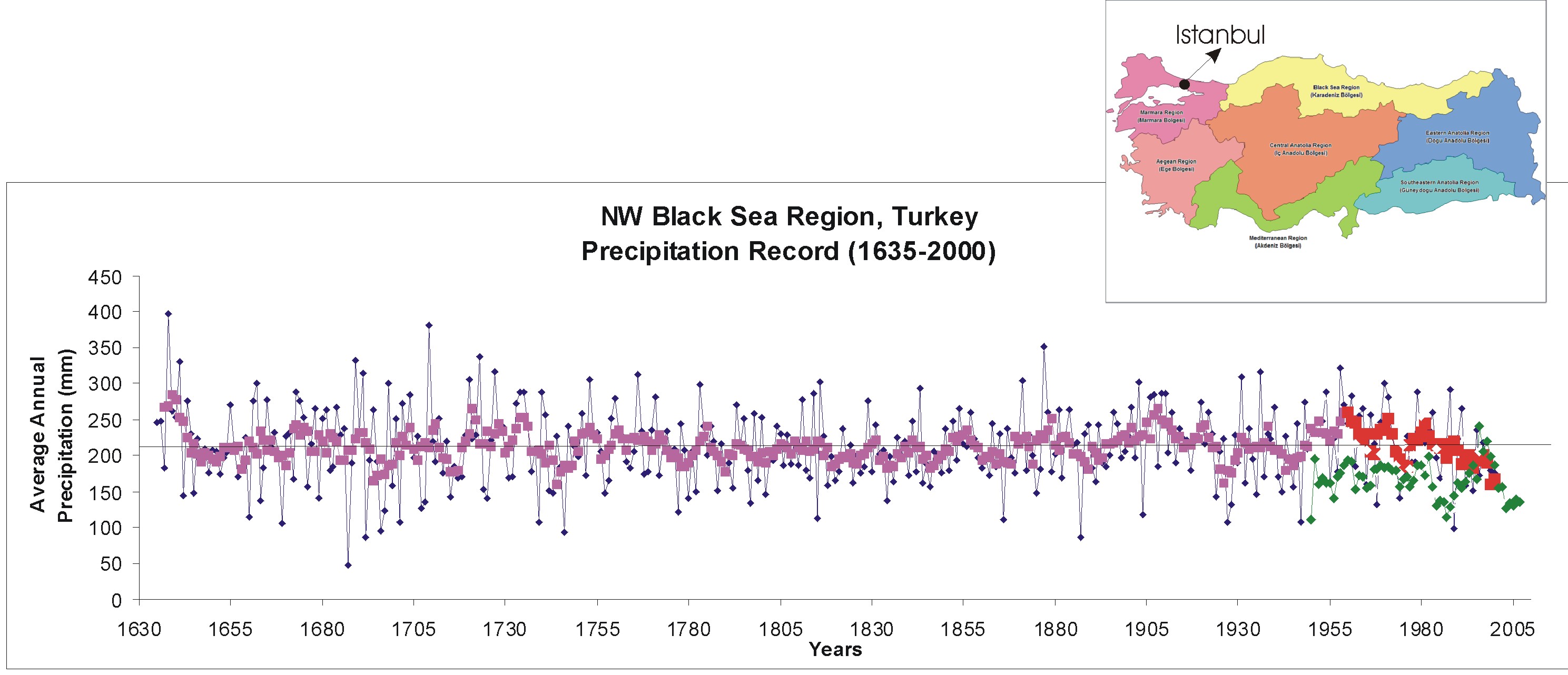
This next graph shows observational spring precipitation data between 1950 and 2007 (shown with green dots) for Istanbul and multi-centennial (1635-2000) spring precipitation reconstruction from tree ring data for the NW Black Sea region in Turkey (pink and red dots show a 5-year running average for precipitation data from tree rings) (data). Multi-centennial tree ring precipitation reconstructions for the Marmara region are not available. Although the observational precipitation record for Istanbul is generally lower than the spring precipitation reconstruction for the NW Black Sea region, both observational and reconstructed data follow a similar trend, except for two unusually rainy springs in 1998 and 2000 in Istanbul. Also note in the tree ring precipitation data that although the amount of precipitation has fluctuated throughout centuries, it has not consistently dropped for more than 3-4 years until the 1970’s. Since then there has been a steady decline until 2000 (the red part of the graph).
In the summer of 2007, temperatures rose over 46°C in many parts of Turkey as well as the entire Mediterranean region. This heat combined with aridity is estimated to have cost Turkish farmers ~$3.9 billion. Turkey’s wheat crop dropped by about 15%. The Turkish Aegean region alone suffered from 30% lower harvest yields in cotton, corn and tobacco and a 50% drop in fig production.
By mid-summer, the drought started to affect major cities. Ankara (~4 million), the capital, suffered serious water rationing this summer (two days on, two days off). Car washing and lawn watering were outlawed within city limits. With the unforeseen burst of the main water pipe feeding the metropolis, the whole city was left without running water for an entire week. Hospitals had to be issued groundwater in tankers, and city officials started to debate whether to delay public school openings until mid-October to contain potential spread of disease. By mid-August, Ankara had only 5% of total capacity in its reservoirs and dams.
 Tuz Gölü, a large salt lake in central Turkey within the Konya Basin, lost half of its water volume in the last four decades. The Konya Basin itself, which hosts a third of all groundwater reserves in Turkey and is the home to eight wetland bird species on the brink of extinction, lost 1,300,000 acres of wetland and witnessed a water table drop of 1-2 meters, also in the last 40 years.
It looks grim.
But not just for Turkey. Even popular vacation areas around the Aegean were hellish this year. Greece had to declare “state of emergency” at least twice this summer: once for forest fires killing over 60 people, burning half a million acres of land, and costing $1.6 billion; and once for drought on the Cyclades Islands due to water shortages.
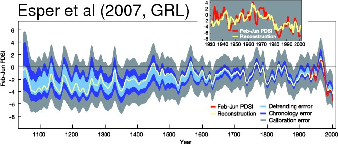
Morocco experienced 50% less rainfall than average this year which will likely result in half of last year’s grain harvest. And because feed prices went up as a result of this drought, Moroccan livestock was also seriously affected. Again, is this an unusual year? Actually not. This next figure, which is from Esper et al.’s (2007) paper in Geophysical Research Letters, shows a significant drop in Feb. – June PDSI (which is a standardized measure of surface moisture conditions after Palmer, 1965) since 1980 in Morocco.
Some speculate that the tragic fires in Greece may have been arson, others say better maintenance of water pipes and anticipation of the coming drought early in the previous winter would have prevented Ankara’s water shortage, and better irrigation systems in Morocco would have mitigated agricultural disaster there.
Though it is “debated” in the US, most people in Turkey consider AGW to be a given. This is generally a good attitude, of course, but it opened the door for some government and city officials to simply blame AGW for drought instead of their incompetence in dealing with it. As a result, the Turkish General Directorate of Disaster Affairs started discussing whether AGW should be listed under “natural disasters” in order to provide better risk assessment and adaptation plans, and to prohibit building new structures in “high risk” areas. Even Al Gore came to visit Istanbul this summer to give a talk at a conference called “Climate Change and its Effect on Life.”
So, is AGW to blame for Mediterranean drought? Although bad land use practices and arson share the blame, AGW is most likely the culprit. Here’s how:
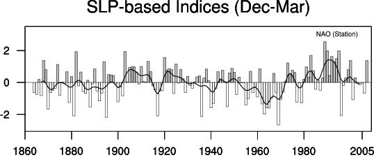
 The North Atlantic Oscillation is an alternation of air masses between polar and subtropical regions of the North Atlantic. When the NAO index (difference between the normalized sea level pressure anomalies in the Iceland and Azores areas, respectively) is in a positive phase, a low pressure system prevails over Iceland and a high pressure system over the Azores. This causes cooler northern seas, stronger winter storms across the Atlantic Ocean, warm wet winters in northern Europe, and cold and dry winters in Canada and Greenland. However, this also causes less rain and reduced stream flow in southeastern Europe and the Middle East. In general, when NAO is in a positive phase, the Mediterranean region receives less precipitation.
 The precipitation pattern in Turkey is well correlated with the phases of the NAO index. For instance Cullen and deMenocal (2000) showed that Euphrates’ spring stream flow varies by about 50% with the NAO index. The NAO index vacillates between negative and positive phases, but its oscillations had a more annual pattern before the 20th century, and since then has become more decadal. More importantly, since the 80’s it has remained in a prolonged positive phase. This is in keeping with the precipitation drop I described for Turkey and Morocco (and the Mediterranean region) in the last several decades.
But do we know that this recent prolonged positive phase in the NAO index is not simply a part of its natural decadal variability? And is this recent positive phase actually related to global warming?
These are tough questions to answer definitively, but it is likely that AGW will continue to keep the NAO index positive because both atmospheric CO2 rise and stratospheric ozone depletion cause a strong polar night vortex. The North Pole is dark and very cold in the winter. This creates a large temperature difference between high latitudes and subtropics. The resulting large pressure contrast forces east-west winds into a stratospheric spiral. And this stratospheric vortex likely causes the NAO to prefer a positive phase. This was first shown by Shindell and colleagues in 1999, and seems to still hold true in the IPCC AR4 runs – although the average signal is smaller. And if it stays that way, southern Europe and the Middle East are likely to continue to get drier.
Thus, the Mediterranean region is at high risk for desertification. Even if 2007 were an anomalously dry year, these disastrous events show us that small perturbations in weather patterns can lead to tragic and costly outcomes. They also show what is in store for this area in the next few decades as global warming progresses. And desert makes more desert. As land is overused and scorched by the hot sun and no rain, it dries up and vegetation cover diminishes due both to drought and wildfires. Lack of vegetation leads to further loss of humidity and increases erosion rates. So, deserts expand even more.
Having said all of this, here is one last thought: if AGW is affecting nearly all latitudes negatively, then we need to wonder where global awareness of this problem stands. The Pew Center Report (2006) found that while over 90% of the population had heard of AGW in countries like the U.S., Germany, France, Britain, Spain and Japan, this dropped to about 75-80% in Russia, Turkey and China and below 50% in Jordan, Egypt, Indonesia and Pakistan (only 12%!). So the peoples in Middle Eastern countries most at risk for growing desertification are barely aware of the problem of AGW. What is even more striking is that of the percentages of people aware of AGW I listed, 70-80% are concerned about it in Indonesia, Egypt, Turkey, Jordan and India; but only 50-60% of U.S. citizens and peoples of China consider AGW to be a serious issue. So the problem isn’t just ignorance, it is also that of profound apathy.
Thanks for that lucid posting Prof Mekik.
This leaves me once again pondering the wider implications of this years Arctic ice melt. The polar region will still be dark and very cold in the winter. But thinner ice means more heat flux between atmosphere and ocean and more water vapour. So it probably won’t be as cold as previous decades.
Anyone know if the vertical temperature difference between surface and stratosphere has a role in forcing the AO into a +ve regime?
Will this years Arctic events force a tendency back to -ve/neutral or reinforce the recent +ve tendency?
Things are not as simple in the Mediterranean. Last spring was one of the more rainiest of the last 50 years in most of the Iberian Peninsula (western Mediterranean), and last summmer one of the less warmest. Furthermore, it is not unusual that seasonal or annual climate anomalies were of different sign in parts of eastern and western Mediterranean.
I just noticed something, so please pardon any misunderstanding.
AGW in the climate science world refers to ‘Anthropogenic Global Warming’. In other areas, it seems to sometimes represent ‘Anti Global Warming’, as in those that refute the scientific consensus in favor of singular or narrowly scoped views.
So in case if there are any others that might be confused by what AGW means, take it in context because there are lots of acronyms in the world.
On the likelihood of prolonged NAO, it just seems logical that if you heat up the planet, the middle will still be hotter that the top and bottom (so history has evidenced). So anything in between the Tropics will be subjected to higher dangerous temperatures in the sense that water and food will continue to be constrained resources.
The rest of the world will be affected also of course. The head in the sand thing, and BAU will be the norm until leaders wake up in force. That just means it will be a more expensive problem as fixing later will cost more than fixing now. Caught in the middle of this are a lot of people that will suffer the fate of decisions made by people that are continuing to ignore reality and common sense. It is unfortunate that many will have to pay a higher price for the decisions of a few.
Thank you, Figen Mekik. You make vivid the interrelations of planetary processes. The natural thought processes of North American habitants indicate to me a positive forcing still. Or perhaps I am using precise words illegitimately. Oceanic inertia may leave inundation to later in the century, but the winds which have whipped around the Greenland ice cap in certain given directions with certain given forces are likely changing now with even the meagerest shrinkage of the cap. Of more imminent concern is the absolute believing of Southwesterners that they will treble their growth in the next two or three decades. I have tried mitigation with a friend located there. “Oh, I wouldn’t worry. We’re already planning desalinization plants on the Pacific to bargain for water rights.” I think I’d have better luck going to Greenland to wave the winds back into their “proper” places.
The situation for the people of Turkey sounds pretty dire – even compared to drought stricken Australia. If the current droughts are truly the result of AGW, then should we interpret this as evidence that the “reduce emissions and eventually stabilize” plans are insufficient and we need some sort of geoengineering to undo the damage we have done?
Also:
@1 – Does anyone have any idea/predictions whether the ice refreeze in the winter will lead to a lower ice mass during winter?
Joe
AGW … AGW ??? ahhhh!! Anthropogenic Global Warming … intuitively obvious eh? silly me, very very clear exactly what it means too eh? ‘anthropogenic’ being a word that I use EVERY day
[edit]
[Response: Actually it is a word we use everyday, and sometimes we forget that others don’t. A simple request is usually sufficient to clear up any misunderstanding. – gavin]
I’d like to know which standardization scheme was used in the tree-ring record.
Can you please post a reference to the treering precipitation record.
Drought conditions seem to becomming very widespread, and areas of flooding becomming smaller in extent (even though they are severe when they do occur.)
Repeating a comment that I made on this site a few months ago:
My conjecture is that as the atmosphere is heating faster than the oceans, that worldwide, the average relative humidity is the decline. The analogy is a bathroom… in order the get a bathroom less “steamy” (without getting rid of the water) is to heat the room (not the water). I assumed this is the reason that the tendency to drought is becomming widespread.
There was no response to my comment last time, hence the repeated post.
Not sure if it helps much, but my understanding from the UK Met Office is that the NAO is broadly neutral or trending negative at the moment – see their chart and explanation on their website:
http://www.metoffice.gov.uk/research/seasonal/regional/nao/index.htmlrecent)
This implies a winter in the UK and NW Europe that will be a bit cooler than those experienced in recent years, with perhaps some more rain for the Med. region. With that in mind, it looks as if there’s a subtropical-like storm developing in the western Med at the moment. These aren’t unheard of, but they are unusual. Watch out for news of how this storm develops later this week.
Regarding Arctic ice, has anyone given thought to the submarine ice off the coast of Canada, and presumably Russia/on the other side, and how this is likely to react/behave as the Arctic warms up? This is relict ice from the last glaciation that has been buried under debris and later submerged as sea levels rose. There’s loads of it, too – many metres thick, over large areas of the sea bed Strikes me as another highly non-linear facet of the system, which could make the local climate response to AGW even more chaotic or confused.
Thanks Gavin, and David I fully understand your point. I’m just gaging by the fact that you have 4.3 million visits on this web site, and guessing that probably not all of those visits are from scientists. I can only speak for one of your visitors :) and I know I’m not a scientist.
@8 Lawrence:
Actually the humidity is predicted to go up, and it has recently been reported that it is indeed going up around the globe. In fact this is one of the main features of (excuse the acronym) AGW — raising the temperature a little causes more water to be held in the air, and since water vapor is a potent greenhouse gas, it raises the temperature still more. By itself, carbon dioxide etc. would not have nearly as big an effect.
Unfortunately simple reasoning by analogy doesn’t work for such a complicated system. The reason for more droughts is partly because the location of precipitation gets changed, with some dry areas tending to get drier while some wet areas tend to get wetter (with more flooding); and second, warmer days and especially warmer nights lead to more evaporation, drying out the soil… while adding to the humidity.
First, I’d like to acknowledge the very patient and constructive support I received from William Connolley and Gavin Schmidt, as well as from anonymous reviewers at RealClimate in writing this post. I learned a lot!
Then I’d like to thank these early posters for their very kind comments! Here are some replies:
Manuel, you are right, not all places were dry and there is a significant difference between the eastern and western Med region when it comes to precipitation patterns. Just check out the observational precepitation trend I show for Istanbul: it looks like it’s getting dryer but 1998 and 2000 got a LOT of rain!!
Yes AGW could satnd for anti-global warming. Thanks for pointing that out John.
David Wilson: As Gavin is pointing out we say anthropogenic every day, all day. It means human induced, but you could look that up too, right?
Aslak Grinsted: The centennial tree ring data is from the World Data Center for Paleoclimatology where the work of Akkemik, Dagdeviren and Aras is published (http://lwf.ncdc.noaa.gov/paleo/recons.html). The spring observational precipitation data for Istanbul is from NOAA National Climate Data Center.
If I am not answering anyone’s specific question, it isn’t because I am ignoring you, it is because I don’t know the answer :)
RE: #2 Maunel
Sadly, Iberian precipitation numbers dispute the value of your anecdote. Total rainfall is decreasing. Total spring rainfall is decreasing.
http://www.worldclimatereport.com/index.php/2007/02/16/the-rain-in-spain/
” … intense precipitation (lines d and e in the figure) is decreasing in all seasons (columns are spring, summer, autumn, winter from left to right) while light precipitation (line b) is increasing. Line a in the figure suggests that total precipitation has generally decreased in all seasons over much of the peninsula.”
” … light precipitation amounts and days with light precipitation are increasing, but the days with and/or amounts of moderate to very intense precipitation are decreasing. Not surprisingly, they also found “there was a decreasing trend in the mean precipitation value per rainy event in every season. This decrease is consistent with the aforementioned increase of the proportion of light rainfall relative to the total.” “
Ethan, consider the source, you’re quoting from a PR site notorious for making things up and twisting facts to fit the story line they’re paid to present. Look them up.
AGW: Perhaps RC could create an acronym glossary. I usually figure them out myself, but sometimes the use of acronyms here becomes overwhelming.
Although bad land use practices and arson share the blame, AGW is most likely the culprit.
Bad land use practices are anthropogenic – human-caused – and operate on a scale that could contribute to regional or global warming. The term AGW thus arguably includes changes due to land-use practices, rendering the sentence confusing.
This would be better: “Although bad land use practices and arson share the blame, CO2 is most likely the culprit.”
Thank you Figen Mekik for a positive article.
Since there are now several people saying that we humans go extinct in about 200 years because of global warming, is it time for a RealClimate article on H2S?
http://www.geosociety.org/meetings/2003/prPennStateKump.htm
http://www.astrobio.net/news/modules.php?op=modload&name=News&file=article&sid=672
http://www.astrobio.net/news/modules.php?op=modload&name=News&file=article&sid=1535
http://www.sciam.com/article.cfm?articleID=00037A5D-A938-150E-A93883414B7F0000&sc=I100322
Here in the Keystone State of Pennsylvania I have noticed something peculiar. The extremes between night and day are increasing, Sometimes I have to put on the heat at night, only to use the air conditioner during the day! Also, my wife got a bad sunburn, one you might get in mid-summer, but it is October. And Denver was seventy degrees one day, and then snowing the next. My analogy is once you lose control of a car, you overcompensate to correct and then you steer in the opposite direction, etc. This is what is happening to the weather patterns. When will we actually “crash”? It may be as soon as next year.
RE: Spencer
Someone can correct me if I am wrong, but I believe that you are talking about specific humidity while Lawrence is talking about relative humidity.
There was a recent (last week?) paper in Nature by Willet et al that indeed confirmed that specific humdiity has increased by ~0.25 g/kg since 1975, and that this increase is most likely due to human influences.
On the issue of relative humidity (Lawrence’s point), I was under the impression that relative humidity remains fairly constant — even with the changing of the seasons. A seminal paper on that issue is Manabe and Wetherald, 1967 (JAS). The prevailing wisdom on relative humidity’s constancy may have changed in recent years, but just last year I heard a prominent climate dynamicist say something along the lines of, “it’s a good approximation, but we still don’t have a satisfactory dynamical explanation for why it is the case.”
However, I am just a geochemist. Perhaps Gavin or one of the other climate dynamicists on this site could elaborate.
Thank you for a very informative and readable comment Madam Mekik.
It’s certainly tough being a Prof, almost as tough as being a member of the RC Group : I had a look at your Prof ratings and your students like you – well done.
I dont post on this site very often because I feel I have nothing of scientific interest to say, but I do post on other sites : principally The Guardian and The Economist.
When I post on global warming I ask basic questions : where are all the mediterranean (and continental) people going to migrate to (to live in a climate where 40+ is the rule rather than the exception takes some doing), where are future food supplies going to come from, and so on. And it is not only drought : geopolitical behaviour is involved too – an example is the Russian position on defending their southern borders and extending their northern ones.
So my point is the same point I made in a recent previous thread about the accessibility of science to the average person on the street using simple numbers and simple measures. Everyone knows that the Dow Jones went down last Friday but nobody pays any attention to the NAO.
If you tell me that the NAO is a good measure then we should broadcast that in all office lifts (elevators) in mediterranean countries and on the front pages of all newspapers, at the same time as refining the models to make the NAO the reference statistic. Now, it may turn out that a refined NAO will be a better statistic, but we have to start somewhere with a good proxy. I am not sure that the problem of inaction on global warming is either ignorance or apathy : I suspect it is more to do with engagement.
People can engage with a number : particularly one that will punish them.
The same considerations apply to an index for sea level rise.
Is it difficult for scientists to come up with a climate index, like the Dow Jones for stock? Is it too un-scientific to do that? Not scientific enough perhaps? Dont want to get your hands dirty with the real world?
One thing is certain, when the City and Wall St. have something to relate to when assessing their own risks then you will see action on global warming, and law suits.
The excellent Mr Hansen (and Gavin) in the Hansen et al 2007 paper and in particular with section 6 started to move down the engagement road. Long may it continue.
Well done RC again, and dont weaken.
Re: #14
Hank, I didn’t look too closely at the rest of the site – I only found the blog post I cited thru Google. That said, nearly all the text I quoted was summarizing (or quoting) Gallego, et al, 2006, described as:
“An article in the recent Journal of Geophysical Research puts the spotlight directly on the rain in Spain as four scientists from the Universidad of Extremadura examined precipitation records from throughout the Iberian Peninsula from 1958 to 1997.”
WCR’s choice of the article and WCR’s (absurd) claim that the findings conflict with the IPCC are silly. But I’ve no reason to doubt the information cited from the recent JGR article, other than that the dataset stops ten years ago. Here’s another source discussing declines in aggregate rainfall in Spain (among other climate change effects and predictions):
http://www.iberianature.com/material/iberiaclimatechange.html
Nick O asked:
Regarding Arctic ice, has anyone given thought to the submarine ice off the coast of Canada, and presumably Russia/on the other side, and how this is likely to react/behave as the Arctic warms up? …
—
I’m no expert on buried relic ice, but I watched AIT at the Holiday Inn Express. Assuming it were to melt rapidly and escape into the ocean, wouldn’t water and earth just fill its former space and cause little to no increase in sea level?
On topic, my wife recently worked in Algeria. They don’t have much agricultural land to lose.
We do need to be more on the QT about acronyms like AGW, NAO and ENSO. We need an acronym list ASAP to be AOK here. It’s OK if you can’t get one up till next AM, but it should be up PDQ. Anyone with an IBM PC that can see HTML should be OK not just in the USA but also in the EC. TNT,
-BPL
Wow, that sounds ominous. So does this: http://www.nytimes.com/2007/10/21/magazine/21water-t.html?em&ex=1193198400&en=e32e766b398790c1&ei=5087 . Good thing the eminent environmental economist Richard Tol assured me on another blog that, “Water scarcity and heat stress have no obvious relationship, as water stress does not mean that drinking water is scarce.”. And here I was beginning to worry that the economists couldn’t chutzpah their way out of this. Never fear!
Hey all, I just stopped by to make the point that I made today in Dr. Mekik’s class that the scientific community needs to move away from the term “Global Warming” and begin to use “Global Climate Change” instead. I am aware that many climate scientists already use this phrase but it still isn’t necessarily “mainstream” at this point. I would like to argue that “Global Climate Change” while more ambigous than “Global Warming” allows for more variations in climate that are taking place to be accepted by those people who aren’t enlightened enough to belive in “Global Warming”. The point was made in class today that the hosts on SportsCenter were dismissing “Global Warming” due to the fact that is was snowing in Denver in October…(gasp!) I contend however, that if the community starts to use “Global Climate Change” more people especially in America where the “debate” still rages will begin to accept the anomolies that we are seeing worldwide that don’t always include warming, drying conditions. Thanks again for the pertinent info Figen, you rule!!!
Very quick..
Glen: that’s a great point, thanks. I’ll ask RC folks if we can make the edit.
Eachran: That is so kind of you to say that you checked my student ratings! I like to teach and I love ocean and climate science, and I think students pick up on both. And pizza. I buy them pizza. :)
Ethan, you write:
> I’ve no reason to doubt the information cited from the recent JGR…
Ethan, that’s my point.
You don’t need a “reason to doubt” — always doubt. Check. There’s far more misinformation out there that Google will find than reliable information. No “Wisdom” button as Cody reminds us.
You can look these sources of up. WCR is well known for biasing and spinning and taking out of context to claim support for their PR.
Even if you find a fact, check for omitted context.
“Trust, but verify.” — R. Reagan.
“The results of the papers were selectively picked up by the World Climate Report (WCR), a publication sponsored by the Western Fuels coal consortium, to assert that current human emissions will not lead to global warming …..” http://www.ucsusa.org/ssi/archive/climate-misinformation.html
There is a good, long, piece in this morning’s NYT (http://www.nytimes.com/2007/10/21/magazine/21water-t.html) about water problems in the American West. More about the problems and what people are doing about them than the “How” of climate of climate change.
Looks like 50 million people are at very high risk of AGW induced drought. We may be past the risk management stage, and into the event response phase.
Re 17
Denver always had a pattern of sharp weather changes, snowing one day, and sunny the next. What has changed is warm moist air from the Gulf of Mexico coming up in the winter to generate large snow events. The blizzards of my childhood, came out of the North as cold, realtivly dry storms. Now, there are some winter storms around Denver that result in more snow. Since this moisture falls east of the traditional snow catch areas, it does little to help the water problems discussed in the NYT piece.
[both atmospheric CO2 rise and stratospheric ozone depletion cause a strong polar night vortex. The North Pole is dark and very cold in the winter. This creates a large temperature difference between high latitudes and subtropics. The resulting large pressure contrast forces east-west winds into a stratospheric spiral. And this stratospheric vortex likely causes the NAO to prefer a positive phase.]
Figen, thanks for a very useful article, could you please spell out a bit more how (a) the CO2 rise and (b) stratoshperic ozone depletion cause a strong polar night vortex? Oh, and what is the polar night vortex? Google finds plenty of references, but all apparently assuming knowledge of the term!
[both atmospheric CO2 rise and stratospheric ozone depletion cause a strong polar night vortex. The North Pole is dark and very cold in the winter. This creates a large temperature difference between high latitudes and subtropics. The resulting large pressure contrast forces east-west winds into a stratospheric spiral. And this stratospheric vortex likely causes the NAO to prefer a positive phase.]
Figen, thanks for a very useful article, could you please spell out a bit more how (a) the CO2 rise and (b) stratospheric ozone depletion cause a strong polar night vortex? Oh, and what is the polar night vortex? Google finds plenty of references, but all apparently assuming knowledge of the term!
Re #18: [Denver was seventy degrees one day, and then snowing the next.]
This is not all that unusual for any place located near a mountain range. It’s happened here (in the Sierra Nevada) several times this year.
With regards to the main article, I still wonder how much of this local change is AGW-related, and how much is simply part of the several thousand year pattern of changes that’ve likely been caused by human agriculture.
Perhaps someone could comment on this question: How many years does it take for some new rainfall pattern or temperature regime to cease being ‘unusual weather’ and be generally considered ‘climate change’? For instance, if summertime day-time high temps have been in the 80 F range for decades, but are now in the 100 + F. range, how many years before this ‘extreme weather’ comes to be normal and that a ‘climate change’ has occurred?
“@1 – Does anyone have any idea/predictions whether the ice refreeze in the winter will lead to a lower ice mass during winter?”
Since the melting season in the Arctic bottomed out there’s not been as much mention of it but I’ve been following Cryosphere Today and it’s clear that the situation is still abnormal. Before this summer their anomaly plot hadn’t gone below -2million sq km, well during the summer they extended it to -2.5 and now to -3! It was only last week that the sea ice area got back up to the previous record minimum (a month late). I wouldn’t be surprised to see a record low maximum this winter. Also I suggested to them earlier this year that they might include a plot of global total sea ice and they have done so (whether it was in response I know not). This is showing a very different trajectory than in previous years.
http://arctic.atmos.uiuc.edu/cryosphere/
I am confused. How do you explain that the NAO index displays a negative trend in the last 15 years, as shown in your plot? Shouldn’t it be pointing up due to AGW?
This is purely anecdotal evidence, but I spent two weeks in Morocco on vacation this spring, and almost everyone I spoke with knew about global warming and knew that it was expected to dry out Morocco.
Nick Gotts (#30) wrote:
If I could hazard a guess…
In the troposphere, greater levels of greenhouse gas tend to raise the temperature as the result of moist air convection from the surface receiving more backradiation. In the stratosphere, above the both the effective radiating level and the tropopause, where one has a negative lapse rate, greater levels of greenhouse gases tend tool result in a net cooling. However, there is an exception: ozone. It absorbs UV directly from sunlight and as such tends to warm the stratosphere. With its depletion the stratosphere tends to cool.
The temperature differential between the stratosphere and the troposphere results in increased circulation of the polar vortex with its strong downward movement near the center, particularly at night as this is when the temperature differential between the surface (with its greater thermal inertia) and higher altitudes within the troposphere will be greatest. However, I would guess that winter is at least as important as night in determining the strength of the vortex.
PS
Here is something interesting (albeit from 2001):
Who somebody is funded by is immaterial. Bad argument. It’s like saying some environmental report was funded by Greenpeace and they’re biased so the paper is no good. Or that the US DOE published something, and the US government is funded in part by engergy companies so everything they put out is biased.
Nick Gotts, thanks for your question and sorry for my slow response. Actually I am going to offer a quick one now and work on a more detailed one to post later. And thanks Timothy Chase for your answer. Basically as the subtropics become warmer, both the tempertaure and pressure gradient between the poles and the subtropics steepens. During long dark polar night (winter) this gradient causes the east-west winds to coalesce into a spiral called the polar night vortex. The more the subtropics warm, the stronger the vortex whcih presumably keeps NAO in its +ve phase.
James, I agree with you. Desert makes more desert and agricultural overuse and degradation is adding to the desertification around the Med. People just want to burn a couple of acres to clear off farm land, but because the vegetation is so dry, the fires go out of control. But arson is arson!
Ps to 36
It would appear that the “Polar Night” is simply another way of refering to the arctic winter, except as it applies to the pole. As such, the Polar Night Vortex refers to the vortex as it exists during the winter, and my statement “However, I would guess that winter is at least as important as night in determining the strength of the vortex” quite literally makes no sense as night and winter are the same thing.
Re. #17
Re. H2S (hydrogen sulfide) extinction possibilities from AGW (human-caused warming).
“Since there are now several people saying that we humans go extinct in about 200 years because of global warming, is it time for a RealClimate article on H2S?”
I personally talked to several peer-review publishing scientists in our building (a national federal climate research lab) on this issue of H2S poisoning possibility in our near future (100-200 years.) One is researching and publishing in this area.
The correct answer according to them (~2 months ago) is “we don’t know…but very unlikely” according to a type of their sort of conscensus. (Note, they are not saying anything like a definite “yes” or “no” and it would be unethical for them to do so with the information they have).
According to them, it is very unlikely that the conditions necessary for H2S tipping points could be reached in this short time period…mainly the idea that for the major oceans to stop overturning enough in this timespan, to let the oceanic oxygen content decrease enough to stop reacting enough with H2S to start letting the H2S go to the ocean surface and go “airborne” in quantity from the ocean depths (I’m doing his from memory, so one of the details might be off a little). Remember, most climate models do not predict the North Atlantic thermohaline circulation (MOC) cutting off for at least 100 years.
http://www.springerlink.com/content/f2glxmjtbh6m2db1/
http://www.agu.org/pubs/crossref/2005/2005GL024368.shtml
That being said, a non-publishing meterologist in this disciplinary area)/(who is also paleoclimatist-leaning in this building) stated to me that we need to keep researching this to make sure…especially as more evidence keeps surfacing (ooooo, I’m full of puns today) that climate can change more rapidly than we had previously thought. So at least several of the world’s top publishing scientists are not losing sleep about this (unlike AGW according to them).
…BUT one was extremely concerned about the ACIDIFICATION OF THE OCEANS (as are a lot of publishing scientists in my building) due to humans putting 30+% more CO2 into the atmosphere and then into the oceans. This makes the oceans more acidic. This can cause problems with coral and plankton and their shells…and the base of the oceanic food chain.
as a matter of fact I know very well what Antropogenic means, and if I didn’t, I expect I am one of the few here who has a personal subscription to the Oxford English Dictionary (OED) on-line to look it up, but even at that I had to wonder what AGW was, GW I knew, AGW was new to me, and the author did, kindly and according to the drill, write it out the first time he used it, all very correct
a famous Canadian thinker, Northrop Frye, said this: “the simple is the opposite of the commonplace”, so I am thinking that wheras Antropogenic is quite absolutely correct, it is maybe just not necessary (?)
just a thought y’unnerstan … Gwynne Dyer has pointed out a disturbing spinoff from the recent fires in Greece (http://www.gwynnedyer.net/articles/Gwynne%20Dyer%20article_%20%20Extreme%20Climate%20and%20Extreme%20Politics.txt) I too have wondered what it may be like when large groups in urban settings begin to feel the pinch – it might not be very pretty
I know this is off topic, not so far in my mind (which thinks that communicating freely may be one of the few antidotes) but off-topic nonetheless, so I will stop lest Gavin [Edit] me again :-)
Re #25
Paul, I fully understand you perspective on ‘Global Warming’ vs. Global Climate Change’.
My perspective is that there are certain special interests that would love it if the scientific community would not use the term ‘Global Warming’.
In my view, when it comes to publicly paid for science, science should serve at the pleasure of public and policy maker understanding.
While this is a web site for science, it is being read by the public and hopefully policy makers. I believe that it is important to use the term ‘Global Warming’ as it is illustrative and accurate to a large degree.
Actually Global Climate Change could mean global cooling also. In this case I would argue that the illustration of the descriptive is ‘very’ important to the presentation and therefore understanding of the audience this science is meant to serve, the public and the policy makers.
#41: Tha author is a she :)
“…both observational and reconstructed data follow a similar trend…”
I don’t understand this inference. I assume that the green dots in your graph are 5-year averages (there’s way too little year-to-year variability for them to represent individual seasons), so the green and red can be compared directly. The green and red seem to have similar changes on the scale of 5-10 years, but the trend from 1950-present in the observed (green) seems to be nearly zero, compared to a massive negative downward trend in the reconstructed data.
Re: #42
John, are the interests you’re referring to the automotive and petroleum industries? I totally understand where you’re coming from with Global Warming and would agree that the term is very much illustrative and accurate to what trends we are currently seeing worldwide. It’s just discouraging for me as an American to know that our country lags far behind the rest of the world when it comes to accepting AGW as a fact. It seems like for whatever reason, non-believers in this country are so quick to point out any climate change that isn’t directly warming as evidence that AGW must not be real. I know that progress is being made everyday, but there are many people in the US that cling so tightly to what the idiot box (TV) tells them that I find it hard to see them changing their opinions until their house on the Beach is swallowed up by rising sea levels.
#44 John Nielson-Gammon: You are right. I was just trying to point out that the ups and downs in both curves (red and green) follow each other. And yes, both the red and green are 5-year running averages. The pink too of course.
#34: viento: I haven’t been ignoring your question. What I get from the figure is the gray bars are positive and the white bars are negative. I don’t know why both 2’s on the axis are labeled -ve. Maybe Gavin or another RC editor can tell us why.
[Response: Fixed. It was like that in the original figure, but there is no doubt that +ve is up. – gavin]
Re. #37, Raplh Smythe:
No, it’s like saying that if a climate science paper was funded by Greenpeace, one should be question the study’s impartiality. There is considerable peer-reviewed evidence that studies funded by organisations that have a financial interest in the study’s outcome are much more likely to reach the desired conclusions than those which aren’t – see, for example, Okike et al 2007; Vartanian et al 2007; and Peppercorn at al 2007.
That’s what happens when you build freeways through the middle of town, and there by cut off and turn nice neighborhoods into shanty towns, and furthermore cut down trees to build car parks. To boot, the place is now ringed by shanty towns. How they have fouled the place.
Re: #11 and #19 Thanks Spencer and Brian for your replies.
Spencer you have not yet given me reason to abandon my conjecture and the bathroom analogy. The same laws of physics apply in my bathroom and the earth. As Brian stated, you did miss the point that I am talking about relative humidity.
My gut feel is that relative humidity averaged out over the entire earth is in the decline (driven by the increased ratio between atmospheric to ocean temperatures). Certainly in Australia, humidity levels are so low that any clouds that do blow in just evaporate away!
I will abandon my conjecture, if worldwide, the amount of low to medium level cloud cover has increased as a result of AGW. I suspect it has reduced. Does anyone have the numbers?
The Mediterranean south west of Western Australia experienced a “step decrease” in rainfall from the mid 1970s continuing to the present. This comprised a loss of early winter rainfall and an overall reduction in average annual rainfall of about 15%. The rainfall reduction has had implications for fire risk, surface and ground water resources and associated implications for agriculture, biodiversity and so on. Attribution of this change in rainfall to AGW has not been determined, but it is a suspect. Further information can be gained from the climate research program website concerned with this matter: http:www.ioci.org.au The 2007 AMOS conference included a session on the SAM for which see http://www.amos.org.au/conf2007/AMOS07_ABSTRACTS.pdf