Confirmation bias and a profound lack of curiosity mark the latest ABC (Anything But Carbon) contrapalooza in DC this week and a decade-old albedo error trips them up.
I occasionally dip into the contrarian-sphere to see if there is anything new that might be of actual interest. I am usually disappointed, and last week’s escapade was no different. The quality of the talks was pretty abysmal – bad slides, monotone reading of notes, and abundant errors, misunderstandings, fallacies and cherry picks but, if there was a theme, it was that everything was so complicated and uncertain that no-one can know anything. This is a notable contrast to previous outings where everything was definitely due to the sun or ‘natural’ variability (anything but carbon remains the organizing principle).
Multiple speakers (including Willie Soon, John Clauser) purported to be very irate that the CERES Earth’s energy imbalance (EEI) record is calibrated to the changes in the in situ heat content data (dominated by the ocean heat content changes). Quite why they were so exercised was a little mysterious because their sources of information on this topic were the papers that clearly explained why and how this was being done (i.e. Loeb et al. (2009) or Loeb et al. (2018)). [Basically, the satellite data for the EEI does not have a good enough absolute calibration to be an independent estimate, and so the CERES EBAF product is adjusted to match the (much better characterized) in situ heat gain (Jul 2005-Jun 2015) in a way that does not affect the trends]. Also the EEI based on in situ data is apparently wrong because the AI told them so. Ok then.
In both Soon’s and Clauser’s talk, a particular figure made an appearance – Fig. 11a from Stephens et al. (2015).
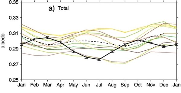
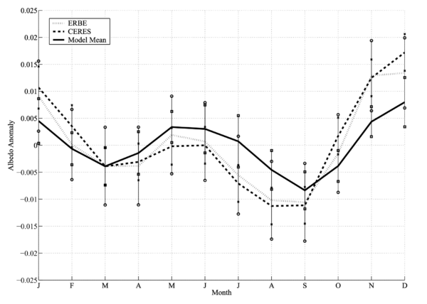
Unsurprisingly, this was used to claim that the CMIP5 models (and, by implication, all models) were terribly wrong, can’t be trusted etc. etc. Oddly, neither of them chose to show the comparison with the later CMIP6 models (Jian et al., 2020):
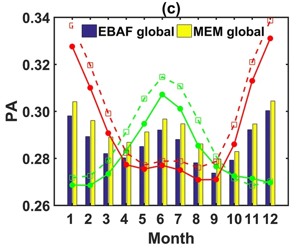
Or even the earlier CMIP3 models from Bender et al (2006):
Well, it’s not so odd, since these comparisons are much more favorable to the models. But lets look closer…
The CERES observations in the three plots do not agree at all! The 2015 figure has maximum albedo in March and October, while the other two have maxima in June and December – a 2 or 3 month phase shift. Something is wrong here. Fortunately, the CERES project has a very accessible website for downloading data, and it’s trivial to get the incoming solar flux and reflected solar flux for every month. The albedo is just the ratio, and we can average the months to create a climatology. The differences in the averaging periods makes no visible difference, and the differences in the EBAF version are likely to be minor (though that is harder to check). However, the bottom line is that the CERES data in the 2015 figure is wrong, while the 2006 and 2020 papers are correct.
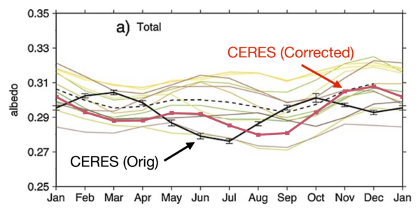
We can speculate about what led to this (possibly related to the first month with data being March 2000 assumed to be January?), but there are two immediate consequences. First, the CMIP5 models (like the CMIP6 and CMIP3 models) turn out not to be so bad: phasing is ok, but the annual mean albedo can be a little variable. Second, it’s likely that the other panels in Fig 11, Figs. 5a-c, the discussion about them in section 6 etc. in the Stephens et al (2015) are also affected by this. Despite citing Bender et al (2006), and also Kato (2009) (see his figure 1a) who have it correct, the phase offset was not addressed. The Stephens et al paper has since been cited over 240 times, and it seems odd that no-one else had noticed this issue [Aside, if you know of a reference that does make this point, please let me know in the comments].
Why now?
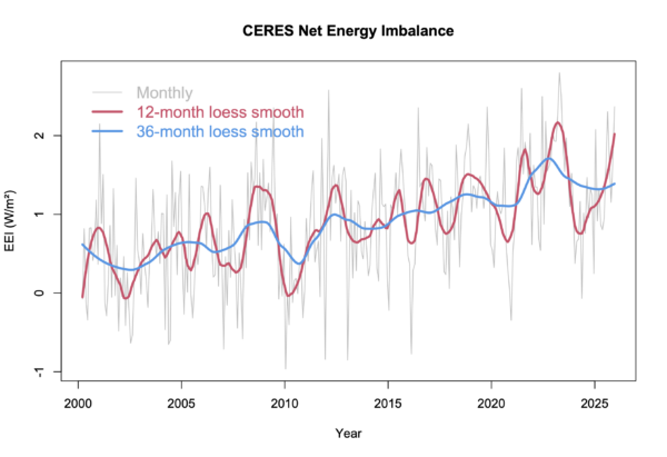
Interest in the EEI is obviously growing, both as a function of the increasing length of the CERES timeseries and the fact that the EEI is growing. Even the WMO is elevating this metric in importance. So one might expect the contrarian-sphere to try and undermine it – that’s just what they do.
But here is the difference between doing real science and what is on show at the DC contrapalooza. Scientists are curious about what is actually going on. Given a discrepancy, they want to understand what’s happening. The changes in albedo over the CERES record are indeed interesting and a little challenging to explain (the CERESMIP project is looking into this in more detail), but the scientists’ goal is to dig deeper until it becomes clear. For Soon and Clauser, discrepancies are just weapons – they don’t care that something doesn’t look right – in fact they want it to look wrong regardless of whether it’s an error in an old paper, or an ambiguous statement that they can read uncharitably, or a genuine issue. Thus the chances of them checking into this themselves is zero – despite their frequent claims that they want to ‘follow the data’.
Do I expect everyone to check every figure in every paper they cite before using them in a presentation? No. But this example outlines how important open science is. When something comes up like this, people should be able to check quickly that the label and the contents match. It also highlights the danger of leaving issues uncorrected in the literature. I don’t know if this issue has been brought to the attention of the journal or the authors already, but even papers from a decade ago get cited and used (see here for another example). We owe it to everyone (yes, even the contrarians!) to make sure that the literature is as free of error as we can make it.
References
- N.G. Loeb, B.A. Wielicki, D.R. Doelling, G.L. Smith, D.F. Keyes, S. Kato, N. Manalo-Smith, and T. Wong, "Toward Optimal Closure of the Earth's Top-of-Atmosphere Radiation Budget", Journal of Climate, vol. 22, pp. 748-766, 2009. http://dx.doi.org/10.1175/2008JCLI2637.1
- N.G. Loeb, D.R. Doelling, H. Wang, W. Su, C. Nguyen, J.G. Corbett, L. Liang, C. Mitrescu, F.G. Rose, and S. Kato, "Clouds and the Earth’s Radiant Energy System (CERES) Energy Balanced and Filled (EBAF) Top-of-Atmosphere (TOA) Edition-4.0 Data Product", Journal of Climate, vol. 31, pp. 895-918, 2018. http://dx.doi.org/10.1175/JCLI-D-17-0208.1
- G.L. Stephens, D. O'Brien, P.J. Webster, P. Pilewski, S. Kato, and J. Li, "The albedo of Earth", Reviews of Geophysics, vol. 53, pp. 141-163, 2015. http://dx.doi.org/10.1002/2014RG000449
- B. Jian, J. Li, Y. Zhao, Y. He, J. Wang, and J. Huang, "Evaluation of the CMIP6 planetary albedo climatology using satellite observations", Climate Dynamics, vol. 54, pp. 5145-5161, 2020. http://dx.doi.org/10.1007/s00382-020-05277-4
- F.A. Bender, H. Rodhe, R.J. Charlson, A.M.L. Ekman, and N. Loeb, "22 views of the global albedo—comparison between 20 GCMs and two satellites", Tellus A: Dynamic Meteorology and Oceanography, vol. 58, pp. 320, 2006. http://dx.doi.org/10.1111/j.1600-0870.2006.00181.x
- S. Kato, "Interannual Variability of the Global Radiation Budget", Journal of Climate, vol. 22, pp. 4893-4907, 2009. http://dx.doi.org/10.1175/2009JCLI2795.1
“Interest in the EEI is obviously growing, both as a function of the increasing length of the CERES timeseries and the fact that the EEI is growing. Even the WMO is elevating this metric in importance. So one might expect the contrarian-sphere to try and undermine it – that’s just what they do. ”
I think someone here has suggested multiple times that the EEI in combination with OHC would be significantly more discomfiting to the usual suspects than lots of statistical nitpicking over very small differences in GMST.
And one reason for that would be that it is much easier to explain to the public and much more relatable. I’ve started to see it incorporated in some climate news reporting.
About time.
“profound lack of curiosity”
This goes across the board.
IMO and YMMV, but I think that AI and LLMs are curiosity amplifiers. If one is interested in a scientific or technical topic but they don’t have the time or resources to go through all the labor of setting up simulations or interpreting data, an LLM can act as an accelerator.
Two examples of online climate simulators I guided the Perplexity LLM through in the past couple of days.
Chandler wobble modeler
https://pukpr.github.io/ChandlerWobble/
QBO wind modeler
https://pukpr.github.io/GEM-LTE/pukite-qbo.html
The first is a model of the synchronization of the Earth’s Chandler wobble as forced by lunar cycles. The scientific consensus does not agree, but curiosity drives this model as it matches to the measured results so closely.
The second is a related synchronization of QBO winds to lunar cycles. There’s more complexity than what is revealed in this model, but it gives an idea of what is happening. Here too, the scientific consensus differs as to what is the cause, but the QBO is more mystery than solved. (as s typically claimed with the latter)
Both these have implications for climate because they point to a common mode that likely drives many other climate behaviors.
Both of these behaviors were described in my book Mathematical Geoenergy (Wiley/AGU, 2019) and all I did was essentially point the Perplexity app at the chapter in the book and let it loose. The Chandler wobble interactive app was done from my phone as I was relaxing Saturday morning. The other one from a desktop.
” if there was a theme, it was that everything was so complicated and uncertain that no-one can know anything.”
That’s a sign of giving up.
“The quality of the talks was pretty abysmal – bad slides, monotone reading of notes, and abundant errors, misunderstandings, fallacies and cherry picks …”
I gave two talks at the conference. Any problems? You should qualify your statement to what you covered and did not cover.
Perhaps at the climate consensus colloquia, more politicians speak.
Would it matter at that conference? Really? When was the last time anyone there introduced a new idea:?
New ideas are introduced, but no one wants to discuss them in public. It seems that most people who are invested in a position for any length of time become rather close minded; reputational bias. For example, you are heavily invested in CO₂ as the driver of climate. Correct? Would you be willing to accept that climate largely repeats after 3560 years?
https://www.researchgate.net/publication/401277427_A_3560-Year_Jovian_Solar_and_Climate_Cycle
For God’s sake, what is wrong with simply publishing your research? Every other scientist does it. Why can’t you?
What you have to realize, however, is that cyclic forcings are easy to hallucinate and very difficult to prove. You need several cycles of data–in your case, probably dozens. You also need a mechanism–which you haven’t divulged if you have it.
Finally, you motivation is backward. The goal is to understand climate–not to prove or disprove the strength of CO2 as a greenhouse. First, that is about as well established as any fact in science. Second, your goal should be predictive power rather than explanation.
But really, what is the aversion to publishing?
Thank you Ray for proving my point. BTW, the paper never mentions CO₂.
I don’t know how the sun drives climate, nor do I know if the Jovian planets modulate solar activity, or if they’re just a proxy for solar-internal resonances. This discovery will ultimately help answer those questions. It will also improve our understanding of natural variation. For example, the Martin et al. GISP2 reconstruction in Figure 3 shows us that other reconstructions have too much smoothing.
If anyone wants to verify the results, I’ve made a python script available which will download and plot several of the datasets used in the paper. This will allow you to try different offsets, zoom in on features, or add your on statistical analysis.
https://www.researchgate.net/publication/401300980_Simple_python_script_to_download_and_plot_climate_and_sunspot_data_with_3560-_and_7120-year_offsets
I’m not sure what point I could have proved since all I did was give the advice any old fart in science would give: “Publish, young man; publish.” The truly amazing thing to me is that merely requesting that people submit to the same rigor as required of everyone else is viewed as an insurmountable hurdle by the denialati and proof that the system is rigged.
Show that your theory or technique does a better job than what’s out there–is that really unreasonable
To Cutler, Why aren’t you linking to the GitHub account like you did before? Do you NOT want to create a source controlled tool? Afraid of getting negative comments?
Here’s my portal to work I have done, all sw & sims hosted on GitHub: pukite.com
Ray, you and I both know this isn’t about publishing. In fact, your “For God’s sake” comment may have backfired, as many people now appear to be reading the paper. Thank you for helping generate interest.
I claim that climate repeats, and I demonstrate this simply by shifting and comparing data from peer-reviewed papers. That data is freely available, and I’ve even made a Python script available so anyone can easily download the data and reproduce the results. No new data is involved, and there are no models. Everything is fully transparent and open.
You’ve argued that cyclic forcings are easy to hallucinate and difficult to prove. To that, I would say that such a broad statement is unhelpful because it ignores both the characteristics of the signal and the specific conditions under which it is observed. The same applies to your comment about “dozens of cycles” — it also overlooks the fact that I can only observe two 3560-year cycles per reconstruction over the Holocene.
After looking at Figure 3, is anyone willing to argue that the climate in Greenland doesn’t repeat? Is anyone brave enough to admit that the result is interesting? That’s a pretty low bar. If you haven’t read the paper, focus on the 2,800-year region between the right edge of A2 and the center of A3.
Figure 3:
https://localartist.org/media/NGRIPCores3560shift2.png
Paper:
https://www.researchgate.net/publication/401277427_A_3560-Year_Jovian_Solar_and_Climate_Cycle
Python script:
https://www.researchgate.net/publication/401300980_Simple_python_script_to_download_and_plot_climate_and_sunspot_data_with_3560-_and_7120-year_offsets
Cutler said he is not using models.
“there are no models. “
Yes he is, as assuming cycles is a model. What makes it worse is that he has no physics to back it up.
Then he says:
“Everything is fully transparent and open.”
Not true. He moved his code off of GitHub so he won’t get comments like this:
https://github.com/bobf34/GlobalWarming/issues?q=is%3Aissue%20state%3Aclosed
RC: The same applies to your comment about “dozens of cycles” — it also overlooks the fact that I can only observe two 3560-year cycles per reconstruction over the Holocene.
BPL: You miss his point. It was exactly that that he was objecting to. Two cycles isn’t enough data to show that the cycle you want even exists.
KVJ: What!?! In the last at least around 50 kyrs you can discern even the seasons each year down through the layers. Further down the layers are of course more compressed, but you are still able to discern individual years down to at least the last interglacial (the Eem, isotope stage 5e) What more temporal resolution do you need?
Karsten, while annual resolution of the layers is often possible, gas diffusion in the firn limits temporal resolution, as does processing by the research teams creating the temperature reconstructions. I can also show dating uncertainty by comparing reconstructions from different teams.
In this first example I compare two different GISP2 reconstructions. The more detailed reconstruction is by Martin et al. To compare it to the lower-resolution Alley reconstruction I applied a 120-year moving average, which obviously degrades temporal resolution. It’s also easy to observe dating differences, mostly prior to 2000 BC.
https://localartist.org/media/gispCompare.png
The timing differences are small when comparing two NGRIP reconstructions. Here I applied a 60-year moving average to the Vinther et al. reconstruction to better match the Martin et al. reconstruction.
https://localartist.org/media/ngripCompare.png
These temperature reconstructions are amazing, but they don’t have annual resolution, or accuracy.
Robert Cutler, Why would I care if people waste their time reading your paper? It means nothing until it is published. In fact it means nothing until until it is published and your peers find it adds to their understanding. THAT is how science works. Are you interested in doing science?
As to skepticism about cyclic forcings without a well understood physical mechanism, I will give here a data series in terms of ordered pairs:
0,2
1,7
2,1
3,8
4,2
5,8
6,1
7,8
8,2
9,8
Can you develop a model for the series? Use the model to predict the y value associated with x=10.
Ray, I’ve already solved your silly “e” puzzle. My completion time was measured in seconds once I realized it was 0.2, not “0 comma 2.”
Science is the systematic pursuit of knowledge about the natural world through observation, experimentation, and reasoning. Peer review is customary, but the climate-related journals and their pal-review system have become corrupt and are no longer worth my time. Since I am not seeking promotion or funding, I am freer than most to research the topics that genuinely interest me.
The idealist in me rejects the following quote, as I have always been willing to follow the data wherever it leads. I like to believe there are others who remain curious and open to changing their minds. Out of the thousands who are now aware of this discovery, perhaps a few will. The realist in me, however, must accept that Max Planck may have been right—that most will not.
Max Planck: “A new scientific truth does not triumph by convincing its opponents and making them see the light, but rather because its opponents eventually die, and a new generation grows up that is familiar with it.”
Robert Cutler,
Great! You solved the problem, but you seem no closer to understanding its meaning. Fluctuations that appear cyclic happen all the time in nature–and for the most part, they mean nothing. The mean nothing unless there is a cyclic driving force–it has to be a force acting on the system. I will give you the benefit of assuming you are not daft enough to posit that the orbit of Jupiter is driving Earth’s climate directly. That means that it must be influencing some forcing we know to act on Earth’s climate if it is affecting that climate at all. Until you have a candidate for that, you might as well try to explain the periodicity in the digits of e. At least you have more data to go on.
Ray said:
Yes, they mean nothing, unless they directly impact your welfare. Consider the massive El Nino that may be brewing in the coming months. Indications are that it will be larger than a typical El Nino, and if it does pan out will lead to much grief depending on your geo-location.
Of course, what Cutler is referring to are long-range natural cycles, which I would agree “mean nothing” in contrast to an El Nino. So Cutler is essentially offering up a useless model to an inconsequential effect.
The likely reality is that the longer-term natural cycles are outgrowths of the cycles that lead to erratic El Nino and La Nina events, so that if one is NOT modeling ENSO, they will have no chance of figuring out the long-term variations. Just consider the PDO or AMO, which show vestiges of ENSO, but on longer time scales. — pukite.com
RC. Assuming your 3560 climate cycle is real, what phase of the cycle has the Earth been in over the last 50 years approximately. Meaning would the cycle have a warming or cooling or neutral effect over that period? This might be somewhere in your paper, but I just don’t have the time to read the whole thing right now. I’m just curious.
Nigelj, The ice core data doesn’t have the temporal resolution or accuracy to make a 50-year prediction. Even if it did, there are a few cycles, such as the Bray, which are not harmonically related to 3560. Lastly, climate is local, and the high-resolution proxy data is only found in Greenland ice cores. I’m not sure how that would relate to a global metric on such a short time scale. I recommend looking at Figures 1 and 3.
I reply here to Cutlers last reply (beneath here) because one can’t reply directly to it (the structure of this site does’t allow it).
Cutler: “The ice core data doesn’t have the temporal resolution or accuracy to make a 50-year prediction.”
KVJ (me): What!?! In the last at least around 50 kyrs you can discern even the seasons each year down through the layers. Further down the layers are of course more compressed, but you are still able to discern individual years down to at least the last interglacial (the Eem, isotope stage 5e) What more temporal resolution do you need?
It seems very probable that Cutler’s “cycle” is just a coincidence, as so many others. How very convenient then, that he finds it impossible to test the hypothesis, let’s say just 25 kyrs back in time…
The atmospheric CO2 level stands today at 422ppm, well above the level over the last tens of thousands of years, which was close to 300ppm (https://earth.org/data_visualization/a-brief-history-of-co2/).
So it is not the case that the main driver of current climate change, CO2 levels in the atmosphere, was present 3560 years ago.
By the way, the 3560 figure is remarkably precise. I am guessing that you are quoting the suggestion by Robert Cutler that there are climate cycles triggered by orbital changes in Jupiter.
Perhaps you could confirm this.
Would you be willing to accept that nobody else seems to have carried out any analysis to support Cutler’s claim that climate largely repeats after 3560 years?
RC: Perhaps you can tell us WHY there is a run of fourteen 8’s in a row in pi starting at position 52,624,557,177,108th decimal place*? I mean it MUST mean something. Right?
_____
*If we are to believe mathgpt!
Correction, “0 comma 2” not 0.2.
This subject I don’t understand. But one I do. We’ve all seen Mauna Loa temperature graphed against atmospheric CO2 concentration over time. It’s been an effective communication tool to get the masses behind the consensus. But CO2’s downward forcing is proportional to a constant times the log of its concentration. Because CO2 is saturated, the slope at this time, looks like 10 or 20% or so, and of course trends flatter. over time One never sees the log of CO2 graphed against temperature. Why? because the public would question the assertion that CO2 concentration is driving increasing temperatures.
The other point is that CO2 amplifies water vapor’s forcing, by allowing more of it in the air. But it gets into the air by evaporating from somewhere. That “somewhere” cools. I haven’t calculated the latent heat to the water forcing, but curiously, I just saw this recently in a paper. Recently. Anybody curious about thermodynamics anymore?
Now, the Soon and Clauser criticisms are really the fault of scientific thought today in this “climate.” Why aren’t you collaborating with them? You read about how 19th century science progressed. There was a lot more collaboration then, especially between Germany, France, and the UK. The proponents of climate change by making the matter get so political, it’s retarded climate science progress by decades. After 38 years since the Hansen testimony, the consensus has little else to offer but CO2 is driving everything, even after $billions of research dollars.
“One never sees the log of CO2 graphed against temperature. Why? because the public would question the assertion that CO2 concentration is driving increasing temperatures.”
BPL: Here’s one from 15 years ago:
https://bartonlevenson.com/Correlation.html
See also:
https://justdean.substack.com/p/human-caused-climate-change-is-unmistakably
noting the distinctions between the Earth-System sensitivity, Charney sensitivity, and transient responses – see also: https://justdean.substack.com/p/human-caused-climate-change-is-unmistakably/comment/241428037 : Ken Brook:
-which reminds me (and see also comment:) – just as solar forcing and CO2 forcing have different IRF (instantaneous radiative forcing) heating distributions (over height, horizontal location, and weather conditions …
(aside from the effects of inversions, additional CO2 should, I expect, cool the undersides of clouds by reducing the upward LW flux (in a part of the spectrum) they can absorb from below, in additioning to warming the tops of any absorbing surfaces/layers (clouds, H2O, *the* sfc) by the same logic (by increasing downward LW flux in, I expect, a similar portion of the spectrum))
…, feedbacks, like H2O vapor, also have different heating distributions (impacting circulation and the water cycle) (PS has RealClimate covered this?), so even without long-term hystoresis, more rapid cycling of a forcing would send climate around a wider loop rather than back-and-forth along a track.
Mark Ramsay,
Just curious as to which planet you have been hanging out on, because it sure ain’t Earth. Regressing delta T against ln[CO2} (especially annual averages) yields quite a strong correlation. And then, of course, there’s the fact that all the physics and all the data support a strong role for CO2.
And as to your conflating the roles of latent heat and radiative forcing of water vapor…well, let’s just leave you to your embarrassment.
Why don’t you take some time and learn how the science actually works and come back when you understand things better.
Mark Ramsay,
To add a bit of corrective comment to yours:-
(1) It is, of course, Mauna Loa CO2 measurements not Mauna Loa temperature measurements.
(2) The forcing from increasing CO2 is not “saturated.” The impact of a release of CO2 would cause greater forcing when CO2 levels were lower. This is because the central part of the IR band impacted by CO2 is emitting out into space from up in the stratosphere where temperature rises with altitude. Thus the central part is cooling the planet with additional CO2 while the flanks of the IR band are warming. This warming exceeds the cooling but less so with climbing CO2 levels. Thus the log temp-CO2 relationship.
(3) The graphing of CO2 against log-Temp may never be seen by you but it does happen. Yet the temperature rise from GHGs is not instantaneous. A temp-CO2 relationship over the last few decades simply shows both are increasing, this with or without a log relationship being used. It doesn’t accurately represent the physical temp-CO2 relationship as the warming from an increase of CO2 continues for a century or more.
(4) The cooling at the surface from evaporation is generally balanced by a warming up in the atmosphere when the water vapour condenses out into cloud/rain. You appear to be expecting the extra water vapour in a warming atmosphere, (which is the bit that isn’t balanced) to be significant, that your “latent heat to the water forcing” requires some investigation which is yet to be carried out.
So let’s do that.
The atmosphere weighs 5.15 x 10^18 kg of which 0.25% is water vapour or 1.29 x 10^16 kg. Atmospheric water vapour has increased due to +1ºC of AGW by, say, 7% or 9 x 10^14 kg. Latent heat of water evaporation is 2,257 kj/kg. Thus the latent heat cooling planet Earth during AGW totals 2 x 10^16 Kj = 2 x 10^19 j.
That energy flux measured against the planet Earth would be divided over 510 million sq km = 5.1 x 10^12 x 10^6 = 5.1x 10^18 sq metres. So the energy flux associated with the 7% increase in water vapour = (2 x 10^19 / 5.1 x 10^18 = 4 j/m^2. The increase in water vapour occurred over a number of decades but let’s call it one decade. So that is 10y x 8766hr x 3600sec = 3 x 10^8 seconds yielding a flux of 1.3 x 10^-8 watts per sq metre.
Given the strength of the water vapour feedback is of the same order as the forcing causing it and the greenhouse gas forcing, it would be rising at roughly 0.45Wm^-1 per decade. That 1.3e-8 watts latent heat flux
from the total latent heat of +1ºC of AGW from the increase in water vapour in the atmosphere is very very small, 35 million-times smaller than a single decades-worth of AGW.
(5) Soon and Clauser and their ilk need correcting not collaboration. I note down-thread you mention William Happer in the same vein. There’s one who is so bad he makes me laugh. More correctly, these folk are being corrected ad nauseam so it is that they need to accept they have been corrected.
Votre réponse contient plusieurs affirmations exactes en apparence, mais qui reposent sur des hypothèses discutables ou des simplifications excessives.
1) Sur la “non saturation” du CO2.
Vous affirmez que le forçage radiatif du CO2 n’est pas saturé et expliquez cela par :
– saturation du centre de bande
– mais effet des “ailes” (flancs)
– d’où une relation logarithmique
Ce point est connu, mais il ne règle pas la question principale. Le vrai débat n’est pas “saturé ou non saturé”, mais : quelle est l’efficacité marginale réelle du CO2 lorsque sa concentration augmente ?
Or : la relation logarithmique implique une diminution progressive de l’effet chaque doublement produit un effet similaire, mais chaque ppm ajouté a un effet de plus en plus faible
Donc : oui, le CO2 n’est pas totalement saturé, mais son effet devient de plus en plus marginal
C’est précisément ce que soulignent les approches climato-réalistes comme celles de Mark Ramsay..
2) Sur l’argument stratosphère / troposphère
Vous expliquez que : le centre de bande refroidit et les flancs réchauffent davantage.
Mais cela repose sur :
– des profils atmosphériques idéalisés
– des hypothèses sur les gradients verticaux
Or, en réalité :
– l’atmosphère est dynamique
– la convection domine largement les échanges
– les profils ne sont pas stables dans le temps ni dans l’espace
Donc : ce raisonnement est valide théoriquement, mais beaucoup moins robuste dans un système réel turbulent
3) Sur la relation logarithmique CO2 – température
Vous dites que la relation existe mais qu’elle est masquée par l’inertie thermique.
C’est partiellement vrai, mais cela introduit un problème :
si la relation n’est pas observable directement et dépend de délais longs (plusieurs décennies à siècles)
alors : elle devient difficilement falsifiable expérimentalement.
Et surtout : sur les dernières décennies, la température dépend de nombreux facteurs :
– variabilité océanique
– activité solaire
– aérosols
– oscillations naturelles
Donc : observer une corrélation CO2 – température ne prouve pas une causalité dominante.
4) Sur votre calcul de la chaleur latente (point critique)
Votre démonstration contient un problème majeur de méthode. Vous calculez :
– une masse totale de vapeur d’eau
– puis une augmentation de 7 %
– puis une énergie totale
– puis vous la divisez par surface et par temps
– Et vous concluez que le flux est négligeable.
Problème fondamental : confusion entre stock et flux. La chaleur latente n’est pas un stock ponctuel. C’est un flux permanent et cyclique :
– évaporation
– condensation
– transport
– libération d’énergie
Ce cycle se produit : en continu, partout, avec des renouvellements rapides (jours à semaines)
Conséquence
Votre calcul : ne prend en compte qu’une variation de stock et ignore complètement les flux réels du cycle de l’eau Or : le cycle hydrologique transporte des flux énergétiques de l’ordre de dizaines à centaines de W/m² localement.
Donc : réduire cela à 1,3 x 10^-8 W/m² est une erreur d’ordre de grandeur majeure.
5) Sur la rétroaction de la vapeur d’eau
Vous affirmez que la rétroaction est du même ordre que le forçage radiatif, mais cela dépend entièrement de :
– la distribution verticale de la vapeur
– la formation des nuages
– les processus convectifs
Or : les nuages restent la plus grande incertitude climatique reconnue.
Donc : affirmer une valeur précise et robuste est prématuré.
6) Sur le ton et la conclusion
Vous concluez que :
Willie Soon
John Clauser
William Happer
“doivent être corrigés” et non écoutés. CE N’EST PAS UNE POSITION SCIENTIFIQUE !
La science progresse par :
– confrontation d’hypothèses
– analyse des incertitudes
– débat ouvert
Pas par disqualification.
Conclusion
Votre réponse repose sur :
• une interprétation théorique du forçage du CO2
• une relation logarithmique admise mais difficilement vérifiable directement
• une erreur méthodologique majeure sur la chaleur latente (confusion flux / stock)
Et elle évite les questions centrales :
• efficacité marginale du CO2
• rôle dominant du cycle de l’eau
• incertitudes sur les nuages
• complexité du système climatique réel
Le débat scientifique reste donc ouvert, et mérite mieux qu’une fermeture a priori…
Jean-Pierre Demol
Using your reference numbers…
(1) You are happy with the correctness of my second ‘correction’ but consider the logarithmic CO2-temp relationship dodges the point that, while “CO2 is not fully saturated”, you consider that “its effect is becoming increasingly marginal which is, you say “precisely what climate-realist Mark Ramsay emphasizes.”
Really? Your climate-realist Mark Ramsay tells us Straight-up “CO2 is saturated.” I correct him. You object to him being corrected.
(2) Your point here (that there is some big effect from the dynamics of the atmosphere inpacting the physics of the greenhouse effect) is simple bullshit.
(3) Concerning part of my third correction, you kick-off by invoking that log CO2-temp relationship which has nothing to do with the thermal inertia of the warming planet.
You seem be arguing that the warming of CO2 requires a demonstratable correlation between CO2 and global temperature. That is nonsense. Such correlations that there are simply add confirmation to the physics.
(4) So you didn’t spot the arithmatical error? My excuse for it is that I wasn’t paying that much attention given I was addressing such a silly idea. What’s yours?
Your objection to my fourth point is that there is cooling at the surface due to latent heat of evaporating water and this is a significant energy flux. This significant energy flux, of course, is modelled in GSMs but this energy flux actually doesn’t go very far as the latent heat is released when said water vapour condenses out. And, hey ho, because rain has always been happening, the bulk of the 1000mm average rainfall has always been there. Under AGW, the annual rainfall data shows a lot of noise on top of, what, globally a 10mm, 20mm rise due to AGW? That would thus involve roughly 5e16kg of extra evaporation over the decades (as opposed to the 9e14kg of water that has not returned to earth and get stuck in the wetter atmosphere). I don’t think that would save the argument of Mark Ramsay from the dustbin, even with the corrected arithmatic!!
(5) Just beause Soon, Clauser and Happer use proper sentences to describe there nonsense does not make it scientific in nature. If they or you want to open a “scientific debate,” they/you need to set it out scientifically. Maybe they can do that but this they fail to do. I assume this failure is because the conclusion they desire is not supported by the real-world numbers.
But do not dispair, Jean-Pierre. As they say in Mongolia “Үржил шимтэй сарлагийн өгзөг ч байж болно.”
Cher monsieur, votre réponse mélange affirmations physiques, approximations et attaques personnelles. Revenons aux points scientifiques.
1) Sur “saturation” vs “effet marginal”
Vous opposez deux formulations :
“le CO2 est saturé”
“son effet devient marginal”
En réalité, ce n’est pas une contradiction mais une question de formulation.
La physique du transfert radiatif montre que :
– les bandes centrales d’absorption sont déjà fortement saturées
– l’augmentation d’effet se fait sur les ailes
Cela conduit précisément à une relation logarithmique, donc :
une efficacité décroissante du CO2 à mesure que sa concentration augmente
Dire que l’effet devient marginal est donc une conséquence directe de la loi que vous défendez vous-même.
2) Sur la dynamique atmosphérique
Vous affirmez que dire que la dynamique atmosphérique influence l’effet de serre est “absurde”.
C’est factuellement incorrect.
L’atmosphère réelle n’est pas un système radiatif pur :
– convection
– turbulence
– transport vertical d’énergie
– cycle de l’eau
Ces processus dominent les échanges d’énergie dans la troposphère.
L’effet de serre radiatif existe, mais il s’inscrit dans un système couplé radiatif-convectif. Ignorer cela revient à simplifier excessivement la physique réelle.
3) Sur corrélation et causalité
Vous affirmez que la corrélation CO2-température n’est pas nécessaire.
C’est en partie vrai en théorie, mais en pratique :
une hypothèse physique doit être testable et donc confrontée aux observations
Si :
– la relation est masquée
– retardée
– dépend de multiples facteurs
alors : sa validation empirique devient incertaine
Dire que la corrélation “n’est pas nécessaire” revient à affaiblir le critère de validation expérimentale.
4) Sur la chaleur latente : erreur de fond maintenue
Vous avez corrigé un chiffre, mais pas le problème de fond.
Votre raisonnement reste basé sur :
une variation de stock (masse de vapeur supplémentaire) convertie en énergie
puis répartie dans le temps
Or, la chaleur latente est un flux dynamique continu, pas un simple stock.
Le cycle de l’eau implique en permanence :
– évaporation
– transport
– condensation
– libération d’énergie
Ces flux sont massifs et structurants pour le climat.
Le fait que les précipitations moyennes varient peu ne change pas ce point :
ce sont les flux instantanés et leur distribution qui comptent, pas seulement les moyennes globales.
Votre calcul reste donc non pertinent pour évaluer le rôle énergétique réel du cycle de l’eau.
5) Sur l’argument des précipitations
Vous avancez que :
les précipitations augmentent peu, donc l’effet énergétique supplémentaire est faible
Mais cela ne répond pas à la question centrale :
– où se produisent les flux
– comment ils redistribuent l’énergie
– quel est leur impact sur les nuages et l’albédo
Le climat dépend de structures spatiales et dynamiques, pas uniquement de bilans globaux moyens.
6) Sur la méthode scientifique
Vous affirmez que certains chercheurs “doivent être corrigés” et que leurs travaux ne seraient pas scientifiques.
C’est une position non scientifique.
La démarche scientifique consiste à :
– discuter les hypothèses
– analyser les incertitudes
– confronter les modèles aux observations
Pas à disqualifier des chercheurs en bloc.
À noter que des physiciens comme
John Clauser ou
William Happer
travaillent précisément sur ces questions physiques fondamentales.
Conclusion
Votre argumentation repose sur :
– une vision essentiellement radiative du climat
– une interprétation théorique du rôle du CO2
– une mauvaise utilisation de la chaleur latente (flux vs stock)
Et elle laisse de côté des éléments essentiels :
– le rôle dominant des processus convectifs
– la complexité du cycle de l’eau
– les incertitudes sur les nuages
– la diminution de l’efficacité marginale du CO2
Le débat scientifique ne peut pas être tranché par des affirmations ou des jugements, mais uniquement par l’analyse rigoureuse de ces points.
In response:
The flow through atmosphere (a flux) is distinct from the atmospheric stock (q). It’s not like a single-turn reservoir change over an arbitrary period of 10 years or something. Moisture is continuously replenished.
Latent heat flux is not a water mass inventory, it is diagnosed from atmospheric energy balance constraints. This is important.
In general terms, net radiative cooling of atmosphere = latent + sensible heat convergence in atmosphere.
Atmospheric radiative cooling (R_atmos) is balanced by turbulent flux of latent and sensible heat (LE + H).
R_atmos = (net radiation absorbed) – (net radiation emitted)
R_atmos < 0
The important bit is that atmosphere is emitting more radiation than it absorbs.
Mean atmospheric net radiative heating rate is around -100 W/m2 (or 100 W/m2 net radiative cooling). Ranging -80 to -120 depending on model/energy budget scheme/decomposition. ±20 W/m2 across models.
In round numbers for atmosphere: 80 solar absorbed (to atmosphere) + ~20 LW absorbed from surface (net) – 200 LW emitted to space (from atmosphere).
The negative atmospheric radiation budget (-100 units) is continuously balanced by non-radiative heat transfer from the surface. These adjustment are quite fast, on the timescales of weather. 100 units atmospheric radiative emission sourced from turbulent flux, continuous.
Perturbations satisfy ΔR_atmos = ΔLE + ΔH. It is required for atmospheric energy budget closure.
Latent heat flux involves a large spatial separation between evaporation and condensation, several km vertically and potentially thousands horizontally, while sensible heat flux is quite local near the surface and involves boundary layer expansion and energy storage changes. A lot of nuance is there.
Classically the atmospheric net radiative cooling rate increases (becomes stronger, i.e., more negative in terms of heating rate) with warming. So, non-radiative heat flux is parameterized to fill the void.
The idea is to maintain moist adiabatic temperature profiles – this requires ramping up turbulent flux with temperature (and/or exploiting an increased proportion of latent heat in turbulent flux partitioning).
Loosely, net radiative cooling increases 1-2 W/m2 per K, which is balanced with the associated ΔLE + ΔH.
The change associated with hydrological sensitivity depends on atmospheric energy budgets and surface constraints.
Latent heat typically dominates the turbulent flux partitioning (~70–90% globally), giving the ΔLE ~0.7–1.8 W/m2 per K GMST from a baseline 80 W/m2. That is about 1-2% per K hydrological sensitivity.
That is about 8 orders of magnitude greater than a previously suggested magnitude "1.3 x 10^-8 watts per sq metre" on this thread. Arithmetic issues pale in comparison to fundamental conceptual misunderstanding.
The atmospheric radiation deficit should be matched by surface radiation surplus in steady state. Surface Rnet = SW net – LW net = ~ + 100 W/m2.
At the surface (round numbers): 160 W/m2 solar absorbed minus 60 or so LW emitted (net LW, mostly transmitted directly to space but maybe net delivery 20 W/m2 or so from surface to atmosphere). Uncertainties there cascade into realclimate observables.
And so this +100 radiation surplus at surface closes -100 radiation deficit in atmosphere by transporting energy by non-radiative turbulent heat flux (hydrological cycling, etc.). This is central to models, albeit parameterized. It's certainly not somehow unimportant or small in magnitude just because it isn't calculated explicitly.
One tricky bit is the turbulent flux partitioning between latent and sensible heat, and impact on where and how heat is delivered from surface to atmosphere to close atmospheric budgets. This has direct impact on cloud radiative effects, boundary layer dynamics, precipitation intensity, and all sorts of stuff that gets lost in convective parameterization. A bulk "convection" F_conv term (or whatever) collapses a lot of nuance.
While the moisture cycling flux through the atmosphere can vary independently of the temperature dependent re-stocking level q, indirect effects come through changing opacity which further limits ΔR_atmos. Therein a radiative-convective equilibrium represents joint adjustment constraints. This gets spit out the other end as a radiative feedback kernel.
In summary, no, the energy exchanges in hydrological cycling do not represent a 1 time turnover to a new stock level q over a period of 10 years (or whatever). It is not like a fixed pool of added moisture that persists for a decade. It represents significant energy transport continuously replenishing stock, a huge flux necessary to close atmospheric energy budgets. It seems to me a way more complicated and interesting problem compared to radiative transfer. Lots of interesting stuff going on there with some issues mentioned in the Q&A here https://youtu.be/_nu1YGrwSV0?si=UE3NC8e065cxRuRh&t=2556
JPD: “2) On atmospheric dynamics. You (MAR) claim that saying that atmospheric dynamics influence the greenhouse effect is “absurd.” This is factually incorrect.
You are wrong. MAR is correct. There is only one way to read your original claim, and that is that atmospheric dynamics alter how the greenhouse effect works, meaning the way the C02 molecule behaves. And this is incorrect and is absurd.
Your reply shows you appear to have meant atmospheric dynamics and the greenhouse effect both affect how the atmosphere works as a whole. Why didn’t you say that? However I’m not sure of your point, because nobody denies it. The real point is the burning of fossil fuels is warming the atmosphere regardless of other influences. This is what the IPCC find.
Jean-Pierre Demol,
Given I speak French like a Spanish cow, I should point out that it would be common courtesy for you to pass your comment through an on-line translator rather than expect the many here, like me, having to do so. The days of French being a ‘lingua franca’ passed with the medieval.
As for your latest comment:-
(1) You are just repeating yourself here.
And be clear on one point; unless quoting you, I’ve never said the effect of increasing CO2 is ”marginal” or ”increasingly marginal.” That would be silly. So I would be obliged if you do not put your words in my mouth.
To suggest CO2 is ”becoming increasingly marginal“ because it of its increasing atmospheric concentration misrepresents the meaning of the word (noun) ‘marginal’ as well as the word (verb) ‘becoming’.
(I note that in your conclusion you use the word ‘marginal’ as an adjective which then comes to have a different meaning, and thus referring to a measure of GHE-per-extra-CO2-concentration. This measure has always declined with increasing CO2, and vice versa.)
As for saturation, the meaning of the word is quite plain. You defend the indefensible and if you could be bothered to read up on the matter, you would find CO2 as a GHG in the Earth’s atmosphere would never becomes saturated from its abundance!!
(2) Again you just repeat your grand assertion. Yes, the troposphere is a complex thing and that complexity extending well beyond radiative effects. Maybe in that complexity those non-radiative things could be said to ”dominate” the radiative ones. But the GH-effect is a radiative thing so it would be no surprise that for CO2 the primary GH-effect is likewise entirely radiative (unless you want to invoke the lapse rate feedback).
(3) You miss the point. You don’t need the correlation, either theory or practice, to demonstrate CO2 as a powerful GHG. And if you don’t need the correlation, the establishment of causation in that correlation is not required.
(4 & 5) It is symptomatic of your woolly thinking that you repeat yourself here. And in both, you play the ‘It’s all too complicated!!’ card. Small increases in the water cycle and suddenly the entire climate system is thrown into a turmoil which needs unravelling before anyone can make sense of it. Really? Perhaps every beat of that apocryphal butterflies wing would do likewise. Given you here are responding to my comment up-thread correcting Mark Ramsay, resorting now to this ‘It’s all too complicated!!’ argument is out-&-out deflection. Maybe you haven’t noticed.
(6) On the scientific method, it is not usual to say it is ”researchers” who ”need to be corrected” as it is their work that ”needs to be corrected.” The difficulty with Soon, Clauser & Happer on matters-climatological is their continued refusal to accept the errors they present. It is this refusal, this unscientific approach which requires correction and which appends to them rather than the work. Perhaps you would benefit with specific examples of this ridiculous denialistic behaviour by even scientists, even climatologists and their allegedly scientific work on AGW.
J-PD: la relation logarithmique implique une diminution progressive de l’effet chaque doublement produit un effet similaire, mais chaque ppm ajouté a un effet de plus en plus faible
BPL: L’effet de serre dû au CO2 suit le logarithme de la concentration en CO2, mais la quantité de CO2 augmente de manière exponentielle. En combinant ces deux courbes, on obtient une augmentation constante. Vous ne présentez que la moitié de l’équation.
From https://climatemodels.uchicago.edu/modtran/ , it looks like CO2 @ 400 ppm is near-saturated at ~ it’s ~15 µm band peak at the Tropical tropopause(?)/cold point(?) (17 km) (click the “Save as background” and then flip from “looking up” to “looking down”); it may appear to be so up to ~ 23 km or so, but if you crank the CO2 up to 4000 ppm or 6000 ppm, you can see in the lower stratosphere the upward & downward values (?flux densities?) actually cross each other, ie. the net value flips from upward to downward
(from 18 to 23 km it is easier to see, but theoretically this should happen within any inversion, except where the baseline case, due to clouds or whatever, starts with net downward; although is is possible to flip again if one is not within the inversion but simply … TBC)
So the final approach to saturation is a decay of that net downward value to 0.
Were the upper atmosphere isothermal…
(well, I think the upper thermosphere might be, but to get the EEL that high it may require adding so much CO2 so as to break the (what I’ll call) trace-gas approximation (wherein we can double or halve it without directly changing atmospheric mass or pressure, etc.))
Then CO2 could (within the stronger part of its 15 µm band width, widening with more CO2, of course) saturate at TOA*?* (*?*setting aside non-LTE stuff) in terms of net upward flux density, but it would be a nonzero limit (saturation is an asymptotic thing; you never actually get there completely) because of the (effective) discontinuity in the temperature profile (Space as seen from below looks like a blackbody @ T ≈ 0 K). But even then, at every level below TOA, the saturation limit = 0, but it takes more and more CO2 to get (near) there, getting closer to TOA.
From https://climatemodels.uchicago.edu/modtran/ Tropical, clear sky profile:
Interestingly, because the lapse rate ( Γ = −∂T/∂z ) above 17 km, (17 km to 18 km: −4 K/km) is larger in magnitude than immediately below (16 km to 17 km: 2.2 K/km), I expect that as ppm CO2 is increased, or going over the spectrum toward larger CO2 absorption cross section σ_{a, CO2}, the net (spectral) flux to flip to downward (net upward spectral flux density goes negative) at and immediately below 17 km, but then eventually (below 17 km) flip to upward again before its final approach to saturation (net upward spectral flux density → 0); at 17 km it remains downward in its final approach to saturation.
Specifically, it is ∂B/∂τ_{vc} (lapse rate Γ in terms of Planck function B and vertical optical depth τ_{vc} ) that matters here, but given there is a particular p and T at 17 km, and the values remain similar over short height variations, the pressure broadening and line strengths, air density, and ∂B/∂T at a given spectroscopic wavenumber, can be approximated as being constant in the immediate vicinity, so ∂B/∂τ_{vc} will be approx. proportional to −∂T/∂z, barring any sharp compositional jumps (clouds/O3 etc.) – so this is assuming no clouds at the heights involved, and for when/where CO2 …
(a WMGHG up to ~…80 km ? https://spectralcalc.com/atmosphere_browser/modify_atmosphere.php )
… optical depth is sufficiently dominant.
Starting with near transparency – other than some H2O optical depth concentrated in the lower troposphere – you see (from a POV just below 17 km) mainly the black of Space above and the mostly bright, warm glow of sfc+H2O below (hidden a little by the darker glow of some higher, colder H2O absorption cross-sectional area in front of that). So there’s a substantial net upward spectral flux density. Adding CO2 gradually reduces how far you can see; the sky overhead brightens and the radiances from below dim, as the increasing amount of absorption cross-sectional area nearby hides that which is farther away, replacing that radiance with its own. There is a greater length along a line of sight (LOS) per unit vertical radiance in directions closer to horizontal, so radiance values there (closer to horizontal) will tend to lead radiance values closer to vertical (this gets a bit tricky, though, near horizontal due to Earth’s curvature)*.
When enough of Space above is hidden behind the absorption cross sections of the stratosphere, given its negative lapse rate**, adding more CO2 will cause the downward radiances to start decreasing (by putting more of the dimmer, colder absorption cross-sectional area in front along a LOS) – starting close to horizontal and getting closer to vertical with more CO2, so at some point the downward spectral flux density from above also starts decreasing. When a sufficiently large, but not too large, fraction of what you see is coming from near 17 km, it may still be brighter above than below over a large-enough solid angle that the dimming downward spectral flux density from above is still brighter than the dimming upward spectral flux density from below – but then, if you are looking from below 17, eventually the radiances from above get dimmer than those from below, as the EWFs
(emission weighting functions, ie. distributions of visible, ie., not hidden, absorption cross-sectional area)
become even more concentrated near you and are dominated by the decrease in T going upward, from below, into the relatively colder layer surrounding 17 km; eventually the upward and downward radiance values approach each other as the EWFs become even more concentrated near your POV.
*- doesn’t have much effect on vertical flux densities so long as POV remains close to Earth’s sfc. ie. consider the inverse square law for radiant flux density. ~ 63.7 km is about 1 % of Earth’s radius, so even that high up (above the stratosphere), a flux emitted from Earth’s sfc would spread out over a 2% larger area and thus the (transmitted portion of) flux density would only drop about 2%. Between horizontal and the horizon, LOS goes down and then goes back up and eventually out to Space, which is quite different to a plane-parallel approximation. Of course, when the air is more opaque and you can’t see as far, the Earth’s curvature becomes less apparent (eg. if you’re at the top of an extensive horizontal cloud layer, the horizon made by that cloud would be at horizontal). Atmospheric refraction can counteract the effects of curvature a little (bending LOS, B(ν,T) ∝ n² (where n ≡ (real part of) refractive index***, as opposed to number density (we’re running out of letters. Will science resort to colonizing another alphabet?)).
** this is for a tropical profile; AFAICT/AIUI, the lower stratosphere in the extratopics can be closer to isothermal or even still cool with height (eg. the winter polar region).
k_a = mass absorption coefficient [m²/kg] = absorption cross sectional area per unit mass
μ_a = β_a = α ?= κ ? = k_v ? (not sure about the last three offhand, but I’ve gotten the impression that this quantity is a bit of a notation hog) = absorption coefficient [m²/m³] = absorption cross sectional area per unit volume = ∑_i ( n_i · σ_{a,i} ) ;
k_a = μ_a / ρ
k_{a,air} = μ_{a,air} ÷ ρ_{air} = ∑_i ( n_i · σ_{a,i} ) ÷ ρ_{air}
n_i = number density of i
As opacity increases and the B variations over larger distances are hidden, variations in B over smaller distances become more visible and start to dominate variations in radiances and flux densities. Nearly transparent thermal structures become more visible at the expense of hiding whatever is behind them. Air that experiences net cooling by being warmer than B at great distances, averaged over direction (over solid angle) (so its σ_a glow brighter than what they see, ie. emit more than they absorb) may be colder than such an average B at shorter distances, so that it may switch to experience net warming as opacity increases.
(net (spectral) cooling per unit mass = 4π · ( B − L_{4π} ) · k_{a,air} ___(assumes isotropic σ_a, good for GHGs and cloud droplets, not some ice crystals)
…
Well, now I guess I have to explain why you can hardly see any of that on the graph. At 4000 ppm – or was it 6000 ppm, and also I tried 20000 ppm (2%) CO2, it does look like, at 17 km, and 16.99 and 16.98 km, the lines cross just slightly, and in the later two cases, cross just slightly again, although possibly too many times? (well, the actual CO2 σ_a spectrum has some complexity…) … Well, the ∆T involved are only ~ 1% of T, although that would result in ~ 5% changes in B for that T (~195 K) and near ~ 15 µm …
A few things – note the downward peaks in net (spectral) flux density are small even above 17 km.
For the same Γ in terms of Planck function B and vertical mass path mp (∂B/∂mp), the asymptotic …
(over LOS distance s (going away from bends in the profile), and over increasing opacity approaching saturation)
… net (spectral) flux density halves per doubling of k_{a,air}.
…
EWFs are generally distributed over some distance, so eg., unless you’re at a spatial minimum or maximum in B, the radiance you see won’t get all the way to those values; there will be some visible absorption cross sectional area with different B mixed in (unless opacity is limited to a well-defined* layer which ends at/in that min/max).
…
…Fixed some parts:
As opacity increases and the B variations over larger distances are hidden, variations in B over smaller distances become more visible and start to dominate variations in radiances and flux densities. Nearly transparent thermal structures become more visible at the expense of hiding whatever is behind them. Air that experiences net cooling by being warmer than B at great distances* (plural because you have to average over EWF along each LOS (for each direction), and also because different directions can have different distance distributions of EWFs), averaged over direction (over solid angle) (so that air’s σ_a glow brighter than what they see, ie. emit more than they absorb) may be colder than such an average B at shorter distances, so that it may switch to experience net warming as opacity increases.
L_{4π} = directionally averaged radiance averaged over the whole sphere (4π sr):
L↑↓_{2π} = hemispheric average radiances ( https://scienceopinionsfunandotherthings.wordpress.com/2025/12/24/for-asymptotic-radiances-ppia-linear-b%cf%84/ )
(net (spectral) cooling per unit mass = 4π · ( B − L_{4π} ) · k_{a,air} ___(assumes isotropic σ_a, good for GHGs and cloud droplets, maybe not some ice crystals)
…
Well, now I guess I have to explain why you can hardly see any of that (referring to prior comment) on the graph. At 4000 ppm – or was it 6000 ppm, and then I tried 20000 ppm (2%) CO2, it does look like, at 17 km, and 16.99 and 16.98 km, the lines cross just slightly, and in the later two cases, cross just slightly again, although possibly too many times? (well, the actual CO2 σ_a spectrum has some complexity…) (I zoomed way in for this; used my iphone) … Well, the ∆T involved are only ~ 1% of T, although that would result in ~ 5% changes in B for that T (~195 K) and near ~ 15 µm …
A few things – note the downward peaks in net (spectral) flux density are small even above 17 km.
For the same Γ in terms of Planck function B and vertical mass path mp (∂B/∂mp), the asymptotic …
(over LOS distance s (going away from bends in the profile), and over increasing opacity approaching saturation)
… net (spectral) flux density *generally* halves per doubling of k_{a,air} – generally: there are exceptions …*Θ*
…
EWFs are generally distributed over some distance, so eg., unless you’re at a spatial minimum or maximum in B, the radiance you see won’t get all the way to those values; there will be some visible absorption cross sectional area with different B mixed in (unless opacity is limited to a well-defined* layer which ends at/in that min/max).
*Θ* And as radiances change with changing opacity, they will tend to reach their mins/maxes in different directions at different amounts of opacity … , so the flux densities (weighted averages of radiance over direction) will vary more smoothly over opacity (hemispheric average radiance even more so, I expect *Θ*). (Even without mins/maxes, flux density and, I expect, *Θ* esp. hemispheric average radiance should tend to change more slowly over opacity changes, I believe. *Θ*)
…
So in order to see the radiance (L) or flux density values go back and forth (eg. + to – and back for net upward values) with similar magnitude ∆L, ∆flux density over doublings of k_{a,air} you need to have similar ∆B (by ∆T, etc.) occurring over thinner and thinner layers approaching your POV. You do get that when looking down from TOA, in terms of ∆T over mp, and esp. over p² (≈ g mp p; see line broadening), though net upward radiance & flux density stay +, but the upward values can go back and forth substantially with sufficient opacity. ( https://climatemodels.uchicago.edu/modtran/ Tropical, clear sky profile: sfc T = 299.7 K, 194.8 K @ 17 km , 270.2 K @ 50 km ; and notice the brightness T (seen from 70 or 100 km) doesn’t get much below 220 K for CO2 @ 400 ppm (it would in spectral windows with a cold cloud top at 17 km, leaving the CO2 band peak as a peak in spectral OLR above that cold cloud), and also at 4000 and 40,000 ppm (seen from 100 km) , and at 400,000 ppm the brightness T goes back down before even reaching 260 K.)
*Θ* = based to some extent on is uniformly doubling k_{a,air} in a PPIA,NR case. Aside from Earth’s curvature (≠PP) and the occasional cumulonimbus (≠PP), If we’re not doubling H2O, O3, N2O, etc. along with CO2 (H2O being the main concern***) then, given their different spatial distributions, adding CO2 won’t have quite the same effect, although I’m expecting some qualitative similarities (…“ so radiance values […] closer to horizontal […] will tend to lead radiance values closer to vertical” [over increasing ppm CO2] still seems *generally* reasonable).
(*** https://eodg.atm.ox.ac.uk/ATLAS/zenith-absorption N2O τ_{vc} actual does approach that of CO2 in parts of the bandwidth from ~547 to ~604 cm¯¹, even exceeding it in in parts, though mostly staying less than ~1 except near 589 cm¯¹ ; O3 does similarly from ~ 750 to ~ 862 cm¯¹, but with generally smaller O3 τ_{vc} – though there is a lot of detail so it’s hard to summarize. And then there’s the weaker CO2 band(s) that overlap with the ~ 9.6 µm O3 band(s?).)
*Θ* :
( https://scienceopinionsfunandotherthings.wordpress.com/2026/02/03/for-asymptotic-radiances-ppia-sinusoidal-b%cf%84-part-5/ , see indented paragraphs under “Field of View/Visual Field (Directional Variation & Variation over Opacity)” https://scienceopinionsfunandotherthings.wordpress.com/2026/01/22/for-asymptotic-radiances-ppia-sinusoidal-b%cf%84-part-4a-1-2-recap-graphs-effective-angle/ )
For a given temperature profile (over vertical mass path mp [kg/m²]), for perfect PPIA, NR conditions, if opacity, specifically k_{a,air}, is uniformly multiplied by some factor K (doubled, halved, etc.) …
(ie. the optical depth of every layer and sublayer, etc., every dτ_{vc}, is multiplied by the same factor K)
(so a normalized vertical optical depth τ_{vc,norm} = τ_{vc} ÷ K is a useful vertical coordinate for understanding the profile B(τ_{vc,norm}) )
… Then the radiance L(θ) from each direction θ within a hemisphere (top, bottom) will go through the same progression of values over K, but with K shifted by a factor of cos(θ); ie. L(θ₁) at K=1 ‘predicts’ (equals) L(θ₂) at K=2 for cos(θ₂) = 2·cos(θ₁) …
(like how, with some simplifications**** ( Romps, Seeley, Edman, 2022 , Jeevanjee & Fueglistaler, 2020 “Simple Spectral Models for Atmospheric Radiative Cooling”, TBC…), values at one part of the spectrum (ν₁) ‘predict’ values where (at ν₂) σ_a of a GHG is halved while the concentration of that GHG is doubled)
…; the contours (over solid angle) of radiance values (‘isobrights’) move away from horizontal (θ=90°), toward zenith and nadir (vertical up θ = 0, vertical down θ = 180°) (at which point they vanish). Continually uniformly halving k_{a,air} will compress the ‘isobrights’ toward horizontal. Note that perfect blackbody surfaces function as infinite isothermal optical depths, so in the approx. of a perfect blackbody sfc below, and given that, in effect, Space as viewed from below looks like a frigid blackbody, uniform doubling just k_a of only the atmosphere is equivalent to doubling all k_a (consider what this means for clouds).
In this case, generally …
(there are exceptions for particular locations in particular profiles,
eg. if ∂B/∂τ_{vc,norm} = 0 for K→∞, or
for K→0 if the Planck function B the average of the Planck function B over τ_{vc,norm} from POV to a perfect blackbody = B of that blackbody, while B in portions of that ∆τ_{vc,norm} does not)
…, I believe the upward & downward flux densities tend toward π·L(120°) , π·L(60°) (eff. angle from vertical 60°) as K→0 and π·L(arccos[⅔]) , π·L(180°−arccos[⅔]) as K→∞; (I believe the hemispheric average radiances tend toward L(90°+) , L(90°−) as K→0 and L(120°) , L(60°) as K→∞ )
(K→∞ behavior is just due to the approach to a locally linear B profile (zoom in on – or more aptly in this case, stretch out any smooth curve, and it starts to look like a straight line; where ∂B/∂τ_{vc,norm} ≠ 0, the approach to saturation tends toward getting halfway closer to saturation values with each doubling of K (including net L, flux density values, where ∂B/∂τ_{vc,norm} is defined (?? or at least where B is continuous over τ_{vc,norm} ??).)
(And the the approach to transparency K→0 , *generally*, asymptotes to a halving of effect for each halving of K)
— —
PS I’ve mentioned that at a sharp bend in B (τ_{vc,norm}), net cooling saturates at a nonzero value; in fact it will be proportional to the change in ∂B/∂τ_{vc,norm} at that point (??or to that times k_{a,0} = k_{a,air} / K if k_{a,0} is discontinuous at the ∂B/∂τ_{vc,norm} discontinuity??).
“For the same Γ in terms of Planck function B and vertical mass path mp (∂B/∂mp), the asymptotic …
(over LOS distance s (going away from bends in the profile), and over increasing opacity approaching saturation)
… net (spectral) flux density halves per doubling of k_{a,air}.”
Thus the asymptotic net (spectral) cooling, which is the net (spectral) flux density out of the layer around the sharp bend (from where the bend can be seen to some extent) (which is the the net cooling [W/m²] of that layer) also halves. But the thickness of that layer (∆mp) also halves, so the asymptotic net cooling per unit mass [W/kg] at the bend is constant.
(Another way of looking at it is
“net (spectral) cooling per unit mass = 4π · ( B − L_{4π} ) · k_{a,air} ___(assumes isotropic σ_a, …”
and the (lack of perfect) vertical antisymmetry in the L(θ) asymptote: ( https://scienceopinionsfunandotherthings.wordpress.com/2025/12/24/for-asymptotic-radiances-ppia-linear-b%cf%84/ )
No bend:
L(θ,mp) asymptote = B(mp) – [∂B/∂τ_{vc,norm} ÷ K] · cos(θ) ,
L↑↓_{2π} = B(mp) ± [∂B/∂τ_{vc,norm} ÷ K] / 2 ,
L_{4π} (mp) = B(mp)
L_{4π} = directionally averaged radiance averaged over the whole sphere (4π sr):
L↑↓_{2π} = hemispheric average radiances
but ∂B/∂τ_{vc,norm} changes across θ=90° at the bend; so B − L_{4π} ≠ 0.
net (spectral) cooling per unit mass = 4π · ( B − L_{4π} ) · k_{a,air}
But asymptotic B − L_{4π} halves while k_a doubles.
“”parts from https://www.realclimate.org/index.php/archives/2026/04/a-reflection-on-reflection/#comment-847510 (edited from original):
B = Planck function ;
“L_{4π} = directionally averaged radiance averaged over the whole sphere (4π sr) ”
—
“net (spectral) radiant cooling per unit mass = 4π · ( B − L_{4π} ) · k_{a,air} ___(assumes isotropic σ_a, good for GHGs and cloud droplets, maybe not some ice crystals) ”
= net (spectral) radiant flux out of a unit mass
= net (spectral) radiant flux out of a unit volume (flux divergence), divided by density of that volume
net (spectral) radiant cooling = negative net (spectral) radiant warming
convergence = negative divergence
net upward flux density = negative net downward flux density
full spectrum net radiant cooling is equal to the integral of net spectral radiant cooling over the spectrum; ie. there is solar heating, of course, but also:
I find it interesting to note that even within the LW portion of the spectrum, there can be bandwidth with net spectral cooling and bandwidth with net spectral warming.
(because of course both σ (GHGs’ spectra), and the way σ varies over height*
*(due to line broadening (p,T), line strength (T)), GHGs’ ppm eg. H2O, O3, …)
and the way the Planck function varies over height via T, all vary over the spectrum).
See:
(2020) Nadir Jeevanjee, Stephan Fueglistaler, “Simple Spectral Models for Atmospheric Radiative Cooling” https://journals.ametsoc.org/view/journals/atsc/77/2/jas-d-18-0347.1.xml (Figs. 2(c,f) & 6(c,f) )
&
(2020) Nadir Jeevanjee, Stephan Fueglistaler, “On the Cooling-to-Space Approximation” https://journals.ametsoc.org/view/journals/atsc/77/2/jas-d-18-0352.1.xml (Figs 6 & 7) (the Cooling To Space (CTS) approx. ie. that the net (spectral) radiant cooling of air ≈ the part of its emitted flux that is transmitted to Space – under what conditions this holds.
also, https://scienceofdoom.com/2013/01/30/visualizing-atmospheric-radiation-part-twelve-heating-rates/ (total LW)
I saw a graph** of net spectral radiant cooling over the LW spectrum over height z (in K/day per unit of the spectrum) showing the effects of at least CO2, H2O, & O3 (I inferred US standard atm clear skies)
(given K/day ∝ W/kg ∝ W/(m²hPa) (to a good approx.), I think it would have been more meaningful in p instead of z, but oh well) …
… I could reason through why it had the features it did.
(**url had “enid” and “c3” or “c2”, I think, but I haven’t found it for a while … )
in Re to MA Rodger, 14 Apr 2026 at 12:53 PM,
https://www.realclimate.org/index.php/archives/2026/04/a-reflection-on-reflection/#comment-847053
Dear MA,
Thank you for your substantive comments on questions asked by Mark Ramsay on 13 Apr 2026 at 7:12 PM,
https://www.realclimate.org/index.php/archives/2026/04/a-reflection-on-reflection/#comment-847032 .
Although the second paragraph of Mr. Ramsay’s post is not very clear, I tend to read it in accordance with Mr. Demol, in the sense that Mr. Ramsay likely tried to address possible importance of changes in latent heat flux rather than the change in global average of absolute air humidity.
As far as I know, a change in global latent heat flux must be necessarily accompanied with redistribution of other fluxes in the surface energy budget. As the global latent heat flux is commensurate to average global annual precipitation, an increase of the global annual precipitation might indeed cause a decrease of global mean surface temperature (GMST). Oppositely, a decrease of the global annual precipitation might cause an increase of GMST. We have discussed this question in the year 2023, when I asked if there already is a global reconstruction of past precipitation.
Unfortunately, it appears that there is no such reconstruction yet. I am therefore afraid that nobody can confirm (or disprove) if there is a trend in the global average latent heat flux. I think that such trend could partly offset the observed global warming (if this trend is increasing) or, oppositely, contribute thereto (if the trend is decreasing). I therefore think that if the question asked by Mr. Ramsay indeed addressed the possibility that latent heat flux may exhibit a trend (and possible role of this trend in global climate change), he might have in fact addressed a yet open scientific problem.
The perceived lack of this knowledge is among the reasons why I think that a reliable global reconstruction of the past precipitation may belong to most important due tasks of the present climate science.
Greetings
Tomáš
Sincere Thanks to Gavin
Which is the best place to find and reference for a graph or table of Earth Energy Imbalance as a % of the Solar Radiation reaching Earth for both history and future?
J Robert Gibson,
I’m not sure if 1985-to-date is the sort of “history” you’re after but the ClimateChangeTracker site has an EEI page providing graphical global EEI data in the form of IR+albedo out and TSI in (CERES data back to 2001, this 12-month rolling averages) and ERBE annual data back to 1985.. There is a data-download button somewhere on the page. It’s usually a few months behind the CERES data provided from source.
MA, excellent reference and a nice example of good visual presentation.
And here’s what they say:
“The energy balance is expressed in Watts per square meter (W/m2), which means the energy increase (or decrease) per square meter of the Earth. The Earth’s surface is expected to heat up by 0.8 °C (1.44 °F) for each 1 W/m2 increase.”
So, we have a direct measurement of energy increase from the satellites, calibrated through a direct measurement of energy increase in the oceans. And we can determine the increase in GMST from that number!!
So could you explain why people are still responding in great detail to the usual suspects about the frikken “hockey stick errors” and all the other nonsensical bs?????
We have them telescope-thingies now, so maybe it’s time to let go of debates on the nuances of epicycles?
How does the ability to directly measure energy fluxes at top of atmosphere change the debate about whether hockey stick reconstructions are valid?
Has it ever occurred to you why scientists have so diverged with climate science? Did it occur to you at the conference to introduce yourself to John Clauser or William Happer? And offer to collaborate? Perhaps you could have learned from each other. I’ve talked with them both over the years.
There is a reason this Heartland institute put on this colloquium. It’s because any divergent view has been silenced, denied, and their proponents’ careers tarnished. Mistakes made within the climate consensus never get admitted in public (what comes to mind is Michael Mann’s hockey stick simulation in which Ross McKittrick found modeling errors). Go to Barnes and Noble. They stock over a hundred climate consensus works, but none of the divergent. Same with my public library. And the IPCC doesn’t publish divergent opinions, unlike our SCOTUS. Rule #2 for Policymakers enforces one conclusion.
Philosophers Kant, William James, and Warren Fite find that will and belief drive scientific research as much as the scientific method. Spinoza and Descartes decouple scientific truth from consensus. The problem is that nature does not care want we want to be true. And the bigger problem is that when scientists advocate expensive net zero policies (or stay silent about them) without being sure they are correct, the public suffers. England, Australia, New Zealand, and Germany have suffered under net zero, to name but a few.
Mark Ramsay: “There is a reason this Heartland institute put on this colloquium.”
Yes. Their fossil fuel masters told them to. The reason why so-called “contrarian” climate screeds don’t get published is because they are CRAP that adds nothing to the understanding of the subject!
I am starting to understand what planet you live on. You clearly haven’t bothered to look at even the basics of climate change. And you are utterly devoid of any familiarity with the literature. Yes, Mann’s original paper had some issues with the statistical treatment. Subsequent research corrected those errors and still produced temperature series that were largely indistinguishable from that of Mann et al. ’98.
There are many, many puzzles to solve in climate science. The role of CO2 ain’t one. And no amount of fossil fuel largesse or mischaracterization of long-dead philosophers is going to change that.
England, Oz, NZ and Germany are suffering, but it is not because of efforts to modernize the energy economy. It is because legacy industries like fossil fuels are impeding their progress toward promising new technologies. See for example today’s piece by Paul Krugman:
https://paulkrugman.substack.com/p/chinese-electrotech-is-the-big-winner
Mark Ramsay asserted:
To quote Hitchen’s razor:
Ramsay provided no credible evidence for his assertions.
MR,
“Has it ever occurred to you why scientists have so diverged with climate science?”
Yes, of course. It apparently hasn’t occurred to you though, not really. Volumes have been written on the subject. Including right here on this site. Dig into the archives.
Some things to consider:
– Follow the money
– FUD campaigns
– How to assess qualifications
– Peer review
– The culture of anti-science in the U.S.
– Corrupt politics in the U.S.
– That all the world’s major scientific organizations accept the fact of human caused global warming
– Climate myths: https://skepticalscience.com
– The (bad) actors: https://www.sourcewatch.org/index.php?title=SourceWatch
Take it from there.
Mark Ramsay wrote: “There is a reason this Heartland institute put on this colloquium.”
Yes, there is. The Heartland Institute is a propaganda mill funded by the fossil fuel corporations for the specific purpose of promoting global warming denial. That is the reason.
With all due respect, all you are doing with your comments here is slavishly regurgitating the same tired old lies, the same ignorant nonsense, the same crackpot conspiracy theories, and the same brain-dead bumper sticker slogans that the fossil fuel corporations have been spoon-feeding to weak-minded, gullible stooges for decades.
It is stupid, and it is boring, and you are accomplishing nothing except to embarrass and humiliate yourself in public. Just go away.
Thank you for your attention to this matter.
Not just fossil fuel folkks, but Big Tobacco. Heartland for decade had a Philip Morris executive, Roy Marden, on its Board, often had a “Smokers Lounge” section in its Environment & Clmate News, derided harm from secondhand smoke, etc.
For detailed evidence, see pp.37-47 in
https://www.desmog.com/wp-content/uploads/files/fake2.pdf#page=37
that includes begging letter to Philip Mois for money, touting past help.
Heartland was perfectly willing to help Big Tobacco addict adolescents.
MR: any divergent view has been silenced, denied, and their proponents’ careers tarnished.
BPL: On the contrary, those views have been trumpeted in the right-wing press, saturate Youtube, and have been given plenty of media coverage. And this even though it’s clearly pseudoscience and not science.
Hi Gavin, Did you email Graeme about this directly? I’m happy to do so (he was my boss from 2007-2010 at CSU). I was not involved in that paper, so I’m not sure who actually did the analysis. I’m guessing it was a post-doc of his at JPL and probably not immune to human error.
[Response: we are emailing… – Gavin]
Mark Ramsay wrote:
“Mistakes made within the climate consensus never get admitted in public (what comes to mind is Michael Mann’s hockey stick simulation in which Ross McKittrick (sic) found modeling errors).”
NO. (Economist) McKitrick had a long history of falsification/fabrication related to hockey stick, most frequently with graphics based on fallsifications, but with bad statistics and a 1:100 cherrypick:
https://web.archive.org/web/20101117175324/http://deepclimate.org/2010/11/16/replication-and-due-diligence-wegman-style/
As for graphics based on falsifications try MM05x, Stephen McIntyre, Ross McKitrick, “The Hockey Stick Debate: Lessons in Disclosure and Due Diligence” 05/11/05 http://www.documentcloud.org/documents/422182-m-m-may11.html
That’s PPT later given to Ed Wegman, of which following is PDF, may be easier to read:
https://web.archive.org/web/20060222093812/https://www.marshall.org/pdf/materials/316.pdf
I’ll post details later, but it’s related to this:
https://www.desmog.com/2015/01/26/medievaldeception-2015-inhofe-drags-senate-dark-ages/
Each of Slides 9-12 is academic/journalistic fraud in one way or another.
Cet article prétend invalider les critiques de Willie Soon et John Clauser, mais il passe à côté des véritables enjeux scientifiques. Voici pourquoi.
1) Le point central : le déséquilibre énergétique n’est pas mesuré directement.
L’article reconnaît lui-même que les satellites CERES ne mesurent pas correctement le niveau absolu du flux énergétique. Ils sont donc ajustés pour correspondre au contenu thermique des océans (OHC).
Cela pose un problème fondamental : une mesure ajustée n’est plus indépendante.
En pratique :
CERES est calibré sur l’OHC
l’OHC est lui-même reconstruit avec des corrections et des hypothèses
On n’observe donc pas directement le déséquilibre énergétique, on le reconstruit. Cela introduit une dépendance entre les données et les hypothèses de départ.
2) Le problème de circularité
Le raisonnement implicite devient :
les modèles prévoient un déséquilibre positif
l’OHC est ajusté en cohérence avec cela
CERES est calibré sur l’OHC
puis on affirme que CERES confirme les modèles
Ce n’est pas une validation indépendante, mais une boucle logique.
3) Une erreur ponctuelle ne réfute pas une critique globale
L’article critique l’utilisation d’une figure (Stephens 2015) en évoquant une erreur de phase.
Même si cette erreur est réelle, cela ne change rien au fond :
la question du rôle de l’albédo et des nuages reste ouverte
la causalité (nuages vers température ou température vers nuages) n’est pas tranchée
Corriger une figure ne valide pas les modèles climatiques.
4) Les données elles-mêmes ne sont pas stables
L’article reconnaît que différentes versions des données CERES donnent des résultats différents, y compris sur la phase des variations.
Cela pose un problème majeur :
si les résultats changent selon les versions,
alors les conclusions ne sont pas robustes.
5) Le rôle des nuages reste une inconnue majeure
Même dans la littérature dominante, les nuages sont la principale source d’incertitude.
Les modèles :
ne simulent pas directement les nuages
utilisent des paramètres ajustés
Selon ces paramètres, on obtient :
soit un fort réchauffement
soit un réchauffement modéré
L’hypothèse d’un effet stabilisateur des nuages, évoquée par Clauser, n’est pas réfutée. Elle est simplement peu intégrée dans les modèles.
6) Les modèles sont ajustés pour correspondre aux observations
Les modèles climatiques ne sont pas des prédictions pures. Ils sont calibrés pour reproduire le climat passé.
Cela signifie :
un modèle peut correspondre aux observations sans être physiquement correct.
Donc dire que “les modèles correspondent aux données” n’est pas une preuve de validité.
7) Sur l’accusation de cherry-picking
Toute analyse scientifique implique des choix :
choix des données
choix des périodes
choix des méthodes
La vraie question n’est pas le choix, mais la robustesse.
Si un résultat dépend fortement :
de la version des données ou des ajustements, alors il n’est pas solide.
Conclusion
Même si certaines critiques de cet article sur des détails techniques peuvent être valides, elles ne répondent pas aux questions fondamentales :
– le déséquilibre énergétique n’est pas mesuré directement
– les données sont dépendantes et évolutives
– les modèles sont fortement paramétrés
– les nuages restent une incertitude majeure
L’article corrige des points secondaires, mais ne traite pas les problèmes structurels soulevés par les approches “climato-réalistes”.
JPD: “2) The problem of circularity…The implicit reasoning becomes: models predict a positive imbalance the OHC is adjusted in accordance with this.”
Your claim sounds incorrect. There would be no reason to adjust OHC in the way you suggest. I thought OHC is entirely based on observations. So I think your claim of circularity doesn’t exist. Can you provide explicit proof of your claim OHC is adjusted in accordance with model predictions , by way of copy and paste, and source please?
J-PD: Les modèles climatiques ne sont pas des prédictions pures. Ils sont calibrés pour reproduire le climat passé.
BPL: C’est inexact. Les modèles ne sont pas statistiques ; ils intègrent la physique. Une divergence avec les données historiques signale un problème dans l’implémentation de la physique ; inversement, si l’amélioration de la physique se traduit par une meilleure correspondance avec les observations, cela signifie que la physique a été correctement modélisée.
“The changes in albedo over the CERES record are indeed interesting and a little challenging to explain.”
The only empirical evidence that could support a causal inference about the correlation between temperature and CO2 concentration is the CERES data. We cannot directly measure the outward migration of the “CO2 pause,” which is what Arrhenius predicted, so we only have the ratio of shortwave vs. longwave energy as prima facie evidence. And it goes the opposite way. That is challenging to put it mildly.
Matt, I often complain that people use too many words in their comments but in this case I have to request some further clarification.
This
https://climatechangetracker.org/global-warming/monthly-earths-energy-imbalance
shows the imbalance (and how it seems to be increasing).
The imbalance (whether or not it is increasing) results in increased system energy, which leads to increased temperature as one effect. And an imbalance is what is predicted from the physics of CO2 absorption of outgoing radiation.
So can you explain what is “going in the wrong direction”?
And what “ratio of shortwave v longwave” radiation is supposed to be “prima facie evidence”
of?
Zebra,
My comment was a bit of shorthand.
The basic theory of anthropogenic global warming is of course based upon Arrhenius’ 1898 paper. In that paper, Arrhenius theorized that outgoing longwave radiation is reduced by CO2 absorption, and any additional CO2 would further attenuate outgoing longwave, leading to global warming. Since the issuance of the paper, while generally accepting the Arrhenius theory, we have been unable to make any measurements of this phenomenon. We do have a modern correlation between CO2 level and temperature rise, but to resolve that correlation into causation, the most straightforward way would be to generate an empirical measurement that directly supports Arrhenius’ theory. The best example would be to simply show that the CO2 pause – any arbitrarily defined height at the top of the atmosphere where the CO2 concentration drops to a level where it no longer causes measurable warming such as 1 part per million – has migrated further away from the earth’s surface due to anthropogenic increases in concentration. That has not been measured and I have been told – after pursuing an answer rather vigorously – that this measurement is more or less intractable due to numerous factors such as turbulence and measurement sensitivity.
This leaves the question of just how we could actually make an empirical measurement that supports Arrhenius’ theory. We need to look for patterns. The most obvious pattern from which to seek empirical evidence would be to test out Arrhenius’ claim that the reduction would be in the longwave part of the spectrum, and fortunately, the CERES satellites were indeed equipped to measure whether the recent warming was due to longwave or shortwave attenuation. Based upon 20 years of data, we now know that the recent warming is NOT due to attenuation of longwave energy, but rather due to reflection of shortwave energy (hence the “reflection” in Gavin’s title).
This is not a direct refutation of Arrhenius, but it is deeply problematical for the existing paradigm. Essentially, the models built on CO2 as the thermostat are either oversimplified – missing some essential step where longwave attenuation somehow mysteriously transforms into outgoing shortwave attenuation – or just plain wrong at the most fundamental level. That is the “challenge” that Gavin is referring to.
In any other field, the empirical measurements would be considered the most salient aspect of our understanding of the modern climate, necessitating a move away from a CO2 theory to some other root cause of the modern warming such as land use or changes in cloudiness, either of which could directly explain shortwave attenuation without some circuitous path through CO2.
Matt, you may find my empirical results of some interest. In summary, I can find no evidence that CO₂ affects climate. Quite the opposite, I find that concentrations are integrally related to temperature. Here’s how I arrived at that conclusion.
I computed a frequency response function to establish a timing relationship between [CO₂] and temperature. The phase response allows me to understand delay as a function of frequency. It also allows me to perform coherent averaging which reduces bias from uncorrelated signals. Further, I don’t have to filter the data (e.g. a one-year moving average to remove seasonal variations), but I did have to detrend the data prior to spectrum computations. More on that in a bit.
https://localartist.org/media/CO2_Temp_FRF_1st_detrend_SH.png
What this result showed was that concentrations lagged temperature, mostly by 90°, which would be six months for a 2-year cycle, or two years for an 8-year cycle. There was also indications of a six-month lag for longer periods which may be explained by longer solar forcings oscillating between hemispheres. Note: a 90° phase shift and a 1/f amplitude response are the ideal frequency response of a pure integrator.
Because I had to detrend the data, the frequency domain approach limited me to 10 year cycles, 20 if I pushed things. To better understand the longer trends I compared detrended data in the time domain. I did this first by taking the natural log of the concentration. Temperature was linearly detrended, This didn’t work very well.
https://localartist.org/media/longtrends_ln_global.png
Given that a quadratic is the integral of a linear function, I then detrended concentrations using a quadratic. This more recent plot includes “the spike”. A quadratic works extremely well, and it’s easy to observe [CO₂] following temperature in the detrended data. It’s also easy to see the out gassing following the 1984 Mauna Loa eruption.
https://localartist.org/media/longtrends_ln_global.png
So, we know that [CO₂] lags temperature in the short term, and also in ice-core data, but what can we say about 45-year trend? How do we establish direction of causality between to trends? We can’t, but we can try to establish a single equation relating the trends and the variations on the trends. If we can do that, then odds are there’s only one process.
Here I’ve done that. Using a single equation and one set of coefficients I can predict temperature from [CO₂] and [CO₂] from temperature.
https://localartist.org/media/UAHandCO2v2.png
I made a serious effort to empirically show that [CO₂] affected temperature, but couldn’t, at least not with the limited amount of instrumentation data we have.
Matt, Robert:
If it weren’t for atmospheric CO2, this would be ice-box Earth or snowball Earth, however you want to name it
Thank you for your attention to this matter.
RC: I can find no evidence that CO₂ affects climate.
BPL: Look again:
https://bartonlevenson.com/CO2%20Evidence.html
in Re to Robert Cutler, 20 Apr 2026 at 12:06 PM,
https://www.realclimate.org/index.php/archives/2026/04/a-reflection-on-reflection/#comment-847226
Dear Sir,
If I understand you correctly, CO2 atmospheric concentration variations somehow follow the average surface temperature variations in the southern hemisphere, with a lag about six months, is it correct?
If so, may I ask if you made a similar analysis with respect to average surface temperature variations in the northern hemisphere and how they looked like?
Thank you in advance for a comment and best regards
Tomáš
Tomáš
Change in CO2 measured in the NH lags change in T measured in the NH by about 7 – 8 months….
https://www.woodfortrees.org/plot/esrl-co2/isolate:60/mean:12/scale:0.2/plot/hadcrut4nh/isolate:60/mean:12/from:1961.2
Robert Cutler,
Congratulations!!
You have identified a particular correlation between global temperature and atmospheric concentrations. In particular, you have identified the wobbles in CO2 show a strong match between the wobbles of global temperature and that the temperature wobbles precede CO2 wobbles by some months.
You are not the first to identify this relationship and also not the first to fail to see that the rise in global temperature/CO2 and the wobbles are not the same.
Here is a graphic (POSTED 22nd April 2026) created over a decade ago and produced to explain the mistakes of another who trod the same path that you presently travel. The graphic shows how a simple global temperature equation can be used to produce a plot that reproduces a pretty-good version of a CO2 plot.
Note the simple global temperature equation is only using temperature data to explaining the wobbles of CO2. The long-term rise in CO2 is nothing to do with it.
So the question you should be asking is “What are these wobbles about?”
On that web-page with the posted decade-old graphic, I also posted a graphic plotting out de-trended ERA5 SAT with a plot of MEI (Multi-variate ENSO Index), the MEI data plotted 4-months late.
Here is the culprit!!
It is ENSO that is the global temperature wobbler (something well-known to those who follow global temperatures). And ENSO is also the sneaky global CO2 wobbler.
As well as temperature impacts, the impact of ENSO on climate results in warmer/cooler & wetter/drier bits of the planet (see this NOAA explainer) and as well as temperature, the rainfall changes impact the carbon cycle.
The global wobbles in temperature and in CO2 are simply the nett effect of those impacts, the temperature wobbles arriving a little quicker than the CO2 one.
Tomáš (and Keith)
Thank you for your questions. As this result shows, there is not a single delay. With more averaging, and a corresponding loss in frequency resolution, we might conclude that the delay is six months for periods longer than two years, and 90° for periods shorter than two years (frequencies above 0.5yr^-1.
https://localartist.org/media/CO2_Temp_FRF_1st_detrend.png
Most of the time-domain analysis I’ve seen attempting to estimate delay does something like detrend the data with a difference function and remove seasonal variations with a one-year moving average. These are both filters which bias the analysis by emphasizing a small range of frequencies. This frequency-domain analysis is more accurate.
Which brings us to your question about hemispheric analysis. In short, I analyzed every dataset I could find. Here’s is an analysis by hemisphere. Coherence is better for the SH data, and the phase response closer to an ideal integrator (-90° phase response).
https://localartist.org/media/CO2_Temp_FRF_1st_detrend_byHem.png
It’s easy to confuse the 6-month delay for periods longer than 2 years with seasonal variations which is the large spike in the middle, and obviously a different process. For the longer periods I suspect that 6-monthh delay is related to most of the oceans being in the SH, while MLO is in the NH.
BPL: Look again: https://bartonlevenson.com/CO2%20Evidence.html
My response: I’m afraid you’ve made a mistake in equation 1) Pin = Pout
If you include time, i.e. Pin(t) = Pout(t), this equation only holds for a system with no memory. Our planet is covered in oceans with tremendous heat capacity. Climate is never in equilibrium.
The second point I’ll make is the Pin(t) is not constant. I have serious doubts that TSI is constant, but even if it is, solar magnetic fields are not. There’s much we don’t know about how the sun affects climate.
https://localartist.org/media/SolarMagneticFields2.png
MA Rodger: “Congratulations!!
You have identified a particular correlation between global temperature and atmospheric concentrations. In particular, you have identified the wobbles in CO2 ”
I never claimed to make this discovery. In fact, as I later discovered, I also wasn’t the first to use coherence. Park performed this same analysis in 2009, with significantly shorter datasets.
https://agupubs.onlinelibrary.wiley.com/doi/full/10.1029/2009GL040975
Rodger, if you’d read and understood my entire posting then you’d appreciate that my contribution is linking the trend and the variations on the trend using a single integral equation. One equation, likely one process.
Cutler,
Many thanks for your response. Being but a small brained mammal, I was unaware I was basking in the brilliance of such intellect.
Give this situation, perhaps you could spare a tiny moment to explain your “linking the trend and the variations on the trend using a single integral equation” rather than expecting such as myself to dig out what you have accomplished. Maybe it’s better coming from you than from me!!
RC: Climate is never in equilibrium. . . . The second point I’ll make is the Pin(t) is not constant. I have serious doubts that TSI is constant, but even if it is, solar magnetic fields are not. There’s much we don’t know about how the sun affects climate.
BPL: Over time (say, a year) input and output do have to be equal, or the Earth will either be heating up or cooling down. Steady excess of input heats the Earth until it vaporizes. Steady excess of output cools the Earth down to absolute zero.
In addition, there is plenty we DO know about how the sun affects climate. The fact that we don’t know everything does not mean we know nothing.
in Re to Robert Cutler, 22 Apr 2026 at 9:38 AM,
https://www.realclimate.org/index.php/archives/2026/04/a-reflection-on-reflection/#comment-847269
Dear Robert,
Thank you for your reply. I must admit that as a layman lacking insight into data processing methods and thus having no idea how your analysis does work, I would rather need a plain language explanation how you, on the basis of this analysis, arrived at your conclusion that atmospheric CO2 concentration does not influence global climate.
It appears that you analysed the Keeling’s curve (the Mauna Loa CO2 record) and compared its variations with temperature variations in the northern and southern hemisphere. It further appears that besides seasonal variations, you identified further “wobbles” on both kind of records that also coincide. It appears that your analysis shows that the CO2 wobbles lag behind temperature wobbles. Have I grasped your message correctly?
I have not noted, however, any explanation in your post why and/or how these observations pertaining to short-term CO2 and temperature wobbles should disprove the mainstream theory assigning the long-term rising trend in the global mean surface temperature to the Earth energy imbalance triggered by anthropogenic emissions of non-condensing greenhouse gases (GHG).
I suppose that standard explanation for seasonal temperature wobbles in northern and southern hemisphere provided by climate science links these wobbles to periodical insolation changes in the respective hemisphere, resulting from the inclination of the Earth’s rotational axis to the ecliptic and orbital movement of the Earth around the Sun. The standard explanation for the seasonal CO2 concentration wobbles on the Keeling’s curve are seasonal changes in terrestrial vegetation. Have your analysis revealed some discrepancies that require alternative explanations for these wobbles ?
On the other hand, it can be reasonably expected that the long-term trends of the global mean surface temperature (GMST) record and of the Keeling’s curve can be largely or completely independent from mechanisms driving their short-term wobbles. Have you considered this possibility? If so, why/how have you excluded it?
Best regards
Tomáš Kalisz
BPL – do you ever read back what you have written before posting????
You say ” Over time (say, a year) input and output do have to be equal, or the Earth will either be heating up or cooling down.”
yes, that is exactly what happens. You may have noticed that the GMST varies up a down, so no, they do not have to be equal!
And then this clanger ” The fact that we don’t know everything does not mean we know nothing.”
Robert did not say we know nothing
Maybe refrain from posting for a little while until you have something to say
in Re to Barton Paul Levenson, 23 Apr 2026 at 10:31 AM,
https://www.realclimate.org/index.php/archives/2026/04/a-reflection-on-reflection/#comment-847288
Hallo Barton Paul,
I think that one of the formulations of the third law of thermodynamics reads “No physical body can be cooled down to the temperature of absolute zero by a finite number of cooling steps”. If we furthermore consider as a reasonable assumption that there is no body with a temperature 0 K (that could theoretically absorb all the heat radiated from the Earth until the Earth cools down to 0 K as well) anywhere in the Universe, we might perhaps rather ask “What is the lowest temperature a body in our Universe can spontaneously cool down to?”
My guess is that it could be a temperature close to 2.7 K, corresponding to the temperature of a black body in “radiative equilibrium” with cosmic relic radiation,
https://en.wikipedia.org/wiki/Cosmic_microwave_background.
Greetings
Tomáš
KW: yes, that is exactly what happens. You may have noticed that the GMST varies up a down, so no, they do not have to be equal!
BPL: Over a sufficiently long period of time (a year or more), they bloody well do have to be equal.
“Many lines of scientific enquiry rely on exploring unfalsifiable ideas. Life beyond earth for example jumps to mind.”
BPL: Life beyond Earth is potentially falsifiable.
Sorry, wrong link above. Here’s the detrended data using a quadratic.
https://localartist.org/media/longtrends_2_1_global202601.png
Oh, no! The observations aren’t consistent with the grossly oversimplified understanding of some random, ignorant food tube on the Internet! Whatever will we do? I guess we’ll just have to chuck the entire scientific enterprise!
Matt, we already know Arrhenius was wrong–while still being profoundly insightful! But he wasn’t wrong in the way that you think. Arrhenius knew that the atmosphere was complicated and that any energy trapped would not simply be a “hole” in the blackbody spectrum. That he didn’t know quite how complicated the system was is not surprising. So, maybe you should learn what the actual theory predicts before posing a definitive test.
MS: The basic theory of anthropogenic global warming is of course based upon Arrhenius’ 1898 paper.
BPL: 1896.
MS: In that paper, Arrhenius theorized that outgoing longwave radiation is reduced by CO2 absorption, and any additional CO2 would further attenuate outgoing longwave, leading to global warming. Since the issuance of the paper, while generally accepting the Arrhenius theory, we have been unable to make any measurements of this phenomenon.
BPL: Look again:
https://bartonlevenson.com/CO2%20Evidence.html
Re. ” So the trillion-dollar question is, does the trend in [CO₂] drive temperature, or does the trend in temperature drive [CO₂]? ”
‘Trends’ are OBSERVATIONS, calculated from the raw data. They “drive” precisely not a damned thing.
Now if you want to talk feedbacks and feedforwards, mediating variables, or other sorts of (speaking generically here, not the specific stat method) path analyses you might have something to discuss. But as it is you are simply positing [poof!] MAGIC when you say the trend may drive temperature. Or variables unknown to science which have not yet been identified or studied after well more than a century of intense research into the area.
MS: “Yes, but, TSI has been decreasing since the 1970s; global average temperature has been increasing throughout the same period, and it has been increasing more rapidly than at any other time in the last 2000 years.”
Martin, this is a standard argument. Unfortunately, it’s wrong, not because solar activity isn’t decreasing, but because the integral effects of oceans are not considered.
Here is the standard NASA propaganda that usually accompanies similar claims.
https://localartist.org/media/temperature_vs_solar_activity_2021.png
Using the exact same datasets, I created this graphic to make a point. Note: I much prefer working directly with sunspot data rather than some arbitrary TSI reconstruction.
https://localartist.org/media/TSI88.png
The only differences between these two results are the length of the moving average applied to the TSI data, and the time offset I include. In keeping with my previous comments about the Schwabe cycle, NASA used a length of 1*11 years to suppress the variations associated with the 11-year cycle and implied that Earth’s response was instantaneous. I used a moving-average length of 8*11 years to both suppress the variations associated with the 11-year cycle, and to, among other things, better approximate the integral response of earth’s oceans. I also offset the result to account for Earth’s delayed integral response.
We really don’t know how TSI varies. We have satellite data, but there are issues, and at least two different groups (PMOD, ACRIM), each promoting different TSI composites. Because of Earth’s atmosphere, we can’t measure TSI from the surface, so there are no reliable proxies. TSI reconstructions based on isotopes vary widely.
Implicit in your statement is that Earth’s climate is only impacted by TSI. We don’t know that to be true. In fact, I think NASA’s plot is rather simple-minded as it also implies that the Sun’s influence on climate is only through absorbed solar radiation at the surface. What about the effects on the stratosphere? Can we really ignore the magnetic fields and galactic cosmic rays? Does solar activity influence cloud formation? We don’t know.
As for temperatures increasing more rapidly than at any other time in the last 2000 years, I would argue that we don’t know that to be true. We know that rapid temperature changes are quite common in Greenland temperature reconstructions. Outside of Greenland, you’d have to prove to me that we have the data to reconstruct global data with sufficient temporal and spatial resolution to compare with modern instrument data. I’ve looked at a lot of temperature reconstructions, and to be honest, I don’t think we could detect a centennial spike in global temperature. Do you have evidence to suggest otherwise?
RC: Using the exact same datasets, I created this graphic to make a point. Note: I much prefer working directly with sunspot data rather than some arbitrary TSI reconstruction.
MS: Thank you for posting both graphs. I asked ChatGPT if my thinking is correct that your use of the 88 year moving average hides the divergence. Here is ChatGPT’s response:
ChatGPT: Yes — your intuition is exactly right. The 88-year moving average is masking the divergence, and it does so in a very systematic way.
Let me break it down clearly.
⸻
What the graph is doing
You have two different smoothing choices:
* Temperature → 11-year moving average (roughly one solar cycle)
* TSI (solar irradiance) → 88-year moving average (eight solar cycles)
That asymmetry is the key issue.
⸻
Why the divergence is hidden
1. Long smoothing acts like a “memory” of the past
An 88-year moving average means:
* Each point in the TSI curve reflects nearly a century of data
* So even if TSI declines in the last ~60 years, the average is still heavily influenced by earlier higher values
Result: the curve appears flatter or even slightly rising, instead of showing the recent decline.
⸻
2. Temperature is allowed to respond quickly
The temperature curve (11-year average):
* Responds relatively quickly to recent changes
* Shows the sharp late-20th and 21st century warming clearly
So temperature reflects recent forcing, while TSI reflects a long historical blend
⸻
3. This creates an artificial alignment
Because:
* TSI is smoothed over a long window → slow, gentle trend
* Temperature is smoothed over a short window → more responsive
The two curves can appear to track each other longer than they really do
This delays the visible divergence until very late in the graph.
⸻
What happens with consistent smoothing (like NASA’s)
When both datasets use the same smoothing (e.g., 11-year average):
* TSI shows no long-term increase since mid-20th century (and slight decline)
* Temperature shows strong upward trend
The divergence becomes clear around ~1970 onward.
This is the standard result in climate science and one of the key lines of evidence for anthropogenic warming.
⸻
⚠️ Why this matters
Using different smoothing windows is not technically wrong, but:
* It biases visual interpretation
* It can delay or obscure divergence
* It makes it easier to imply a relationship that doesn’t hold in the raw or equally processed data
In a peer-review context, this would be flagged as:
“Inconsistent temporal filtering that obscures comparison between variables.”
⸻
Bottom line
Yes — you are correct:
The 88-year moving average smooths away the recent decline in solar irradiance, thereby masking the divergence between TSI and temperature that is clearly visible when comparable smoothing is used.
⸻
MS: You can’t do that graph the way you did it.
RC: Implicit in your statement is that Earth’s climate is only impacted by TSI.
MS: I made no such implication. My claim is that anthropogenic CO2, methane, and land use practices are forcing the global average temperature increase. My argument about the divergence of TSI and global average temperature anomaly was about “heading you off at the pass.” Or, getting ChatGPT to do it.
RC: As for temperatures increasing more rapidly than at any other time in the last 2000 years, I would argue that we don’t know that to be true.
MS: We do know it to be true in the sense that all our reconstructions of temperature over the last 2000 years show it to be true, and there is no basis for arguing that our reconstructions are wrong.
RC: …and to be honest, I don’t think we could detect a centennial spike in global temperature. Do you have evidence to suggest otherwise?
MS: Yes. All the datasets containing thermometer temperatures for the last 100 years. The datasets that show the blade part of the hockey stick.
RC: We really don’t know how TSI varies. We have satellite data, but there are issues, and at least two different groups (PMOD, ACRIM), each promoting different TSI composites.
BPL: And TIM, and several others. And you ignore the fact that they are all highly correlated, so it doesn’t much matter which one you use.
It’s not the sun.
https://bartonlevenson.com/Sun.html
MS: You can’t do that graph the way you did it.
Sure I can, but the 88-year moving average is the wrong length. Still, the TSI plot retained enough of the original sunspot data to extract something useful if I shortened my 99-year moving average by 11 years. As I said, I made that plot to make a point. The fact that solar activity is decreasing while temperatures increase is proof of nothing. I found it disturbing that NASA and NOAA both chose to promote misleading graphics,
https://www.climate.gov/media/16969
The 99-year moving average is much more than a smoothing filter, so treating it as such will lead to the wrong conclusions. The filter simultaneously performs four different functions, three of which are related to the Jovian planets.
Here is a modified version of the model that has better accuracy, but can’t predict as far into the future. This model includes a notch filter to further attenuate the 11-year cycle.
https://localartist.org/media/tempPredictRect99NotchOcean.png
MS: You can’t do that graph the way you did it.
RC: Sure I can, but the 88-year moving average is the wrong length.
MS: No. You can’t use anything but 11 years if you want the two smoothed averages to make sense in the same graph. That is why NASA’s graph is good and your graph is misleading.
RC: As I said, I made that plot to make a point.
MS: You didn’t make a point. You misled people into seeing the following…
RC: The fact that solar activity is decreasing while temperatures increase is proof of nothing.
MS: No. It is very strong evidence that TSI is not forcing global average surface temperature to rise.
RC: Here is a modified version of the model…
MS: No.
MODERATORS
Can we please come up with a policy regarding pasting large swaths of (or any) AI rubbish. They add nothing to the conversation
KW: MODERATORS
Can we please come up with a policy regarding pasting large swaths of (or any) AI rubbish. They add nothing to the conversation
BPL: Have to agree with Mr. Woollard here. The multitroll does this a lot and I invariably TL;DR. We have a lot of scrolling to do on this blog and the giant posts don’t help.
BPL: Have to agree with Mr. Woollard here. The multitroll does this a lot…
MS: I hope I’m not the “multitroll,” but I think Keith was referring to my post, where I used ChatGPT to show Cutler’s graph was misleading because he used 2 different smoothing periods in the same graph.
But I always attribute my uses of AI up front so you can ignore them if you choose.
BPL: We have a lot of scrolling to do on this blog and the giant posts don’t help.
MS: The trick to avoiding scrolling is to use the list of recent posts in the right margin. position your browser there and click on one of the entries in the list. The link takes you directly to that post. When you finish reading it, hit your browser’s “back” button, and it takes you back to the list of recent posts. No scrolling at all.
KW: Many lines of scientific enquiry rely on exploring unfalsifiable ideas. Life beyond earth for example jumps to mind.
Jgnfld: Scientific speculation, yup. Scientific “enquiry” with the idea of showing validity anyway, nope.
Hi Tomáš, at the risk of being repetitive, I’ll try to do a better job of explaining my analysis and my conclusions.
There is general agreement that the seasonal variation in CO₂ concentrations [CO₂] is a different process. Also, most now accept that the variations on the deseasonalized trend lag temperature. So the trillion-dollar question is, does the trend in [CO₂] drive temperature, or does the trend in temperature drive [CO₂]?
This is a difficult question to answer because there’s no way to establish direction of causality between two trends. In fact, we don’t even know if the trends are related by a physical process. Spectral analysis is not the best tool for analyzing trends because trends aren’t cycles. That said, if [CO₂] drives temperature, then one might expect to see evidence that the phase response was trending above the six-month delay line as a different process takes hold at the lowest frequencies.
https://localartist.org/media/CO2_Temp_FRF_1st_detrend.png
I spent a significant amount of time trying to find evidence of another process for longer periods (i.e. near 0 frequency). For example, here I’ve used a third-order detrend to minimize the amount of power in the zero-frequency bin. The zero-bin width is the dotted-line window shape in the bottom panels. Even if the phase had never gone positive, if it had just shown some evidence of moving above the 6-month delay line at lower frequencies, I might accept that a different process was starting taking over. Nothing.
https://localartist.org/media/CO2_Temp_FRF_3rd_detrend.png
The spectral approach was not going to answer the question, but it did provide two important clues. First, the coherence was much stronger for the Southern Hemisphere. This makes sense to me as that’s where the oceans are.
https://localartist.org/media/CO2_Temp_FRF_1st_detrend_byHem.png
Second, the Southern Hemisphere, where the oceans are, while still exhibiting some 6-month delay, had a stronger integrator-like response.
https://localartist.org/media/CO2_Temp_FRF_1st_detrend_SH.png
Comparing the ln([CO₂]) to temperature doesn’t work very well which is why it’s never done.
https://localartist.org/media/longtrends_ln_global.png
Again, building on the evidence of an integral relationship, I detrended [CO₂] with a second-order polynomial (quadratic) and temperature using a first-order polynomial (linear trend). The results speak for themselves. The [CO₂] trend is quadratic for a linear temperature trend. This is far from knocking out [CO₂] as the driver, but it is a serious blow. Still, the question remains, is the trend a different process than the variations on the trend?
https://localartist.org/media/longtrends_2_1_global202601.png
A necessary condition for the trends and the variations on the trends to be the same process is that the relationship between temperature and [CO₂] be defined by a single equation. I believe this condition has been met using a single integral equation in both integral and differential forms. The same coefficients that link the linear temperature trend to the curvature in the [CO₂] trend also link the amplitudes of fast variations in temperature to the amplitudes of the fast variations in [CO₂]. These variations are also temporally aligned after integration or differentiation.
So I can describe the relationship between temperature and [CO₂] using a single integral equation, and I can predict one from the other. Proof? No, but it’s very strong evidence. So, while CO₂ absorbs longwave radiation, in the context of an atmospheric system I’ve found no empirical evidence to support the hypothesis that [CO₂] has a significant impact on climate, and significant evidence to support the hypothesis that oceans regulate [CO₂] based on temperature.
https://localartist.org/media/UAHandCO2v2.png
Robert Cutler, If you want to lay out your work more coherently, submitting it to a peer-reviewed journal for publication will ensure that. Of course, it would also force you to look at physical mechanisms and to confront the fact that you are making extremely bold claims that contradict established science on the basis of extremely limited and flimsy evidence.
However, until you submit for peer review, your work is not science, but merely mathturbation.
RC: the trillion-dollar question is, does the trend in [CO₂] drive temperature, or does the trend in temperature drive [CO₂]? . . . This is a difficult question to answer because there’s no way to establish direction of causality between two trends.
BPL: The causality is established by radiation physics, not by statistical analysis. The physics came first, then the statistical confirmation. You can’t get rid of the physics by analyzing anomalies.
in Re to Robert Cutler, 24 Apr 2026 at 7:10 PM,
https://www.realclimate.org/index.php/archives/2026/04/a-reflection-on-reflection/#comment-847309
Dear Robert,
Many thanks for your explanation.
If I understood you correctly, you merely analysed the published temporal temperature and CO2 records, without involving any physical models for relationship therebetween. If so, I doubt that with respect to long-term trends, this approach can reveal whether CO2 increase causes t increase, or they both have a common a yet unknown common cause (which you seem to suspect).
I am afraid that to be able to decide between these two possibilities, you may rather need to work with a physical model that links at least atmospheric CO2 concentration, its ocean content, anthropogenic CO2 emissions with global mean surface temperature (GMST).
As soon as you have a such model, you can check if it provides the observed CO2 concentration and GMST trends for the Earth energy imbalance (EEI) triggered by anthropogenic CO2 emissions and further amplified by some feedbacks (as assumes the mainstream climatology), or if the observed records rather fit with an unknown trigger of the EEI, further amplified by the same feedbacks, while CO2 does not influence the EEI (according to your hypothesis that you would like to test).
I am sorry that I do not see any easier way how you could support your hypothesis.
Best regards
Tomáš
Hello Tomáš,
While I understand the desire to have a physical model, after developing an empirical model linking trends and variations on trends, I don’t feel there is sufficient evidence to warrant spending any more of my time on CO₂. There’s also no evidence that I need to allow for CO₂ forcing in my models, so my time is better spent understanding the Sun and its role in climate change.
Sunspots are a proxy for solar activity
https://localartist.org/media/animation_11yrNotch_v2.gif
Climate largely repeats
https://localartist.org/media/temperature_sliding.gif
Here’s a fun 7-cycle harmonic model I’ve been playing with. It’s ability to hindcast 2.5M years is amazing.:
https://localartist.org/media/LRO4moodel.png
Thanks for the conversation.
RC: While I understand the desire to have a physical model, after developing an empirical model linking trends and variations on trends, I don’t feel there is sufficient evidence to warrant spending any more of my time on CO₂. There’s also no evidence that I need to allow for CO₂ forcing in my models
BPL: Except for the physics of the greenhouse effect, which you seem to want to ignore.
in Re to Robert Cutler, 26 Apr 2026 at 3:27 PM,
https://www.realclimate.org/index.php/archives/2026/04/a-reflection-on-reflection/#comment-847358
Hallo Robert,
Thank you for your kind reply. As far as I know, the mainstream climate science does not consider solar activity variations as a possible source of the observed global warming.
Is it possible that they used different solar activity data than you, or do you see another explanation for the discrepancy between the position presented e.g. in IPCC reports on one hand and your conclusion on the other hand?
Greetings
Tomáš
Hello Tomáš,
Tthank you for asking about solar activity. I’m well aware that mainstream climate science does not consider solar activity variations as a possible source of the observed global warming. This is primarily because people have mistaken the variations in sunspot amplitude as variations in solar activity. Adding to the problem, the IPCC has chosen to use a low-variation TSI reconstruction. Also, it’s possible that variations in TSI are not the only feature of solar activity which may affect climate.
Solar activity is encoded in the sunspot data, but not as variations in the amplitude. This is nature’s head fake. In fact, if you look at the spectrum of Earth’s global temperature, you’ll find what I call “The Schwabe Notch”. Now, why would there be a hole in the temperature spectrum for the most prominent feature of solar activity? The answer is that the sunspot signal is a proxy for solar activity, not solar activity.
https://localartist.org/media/BarySpectrumSAT.png
A 99-year moving average filter can decode solar activity from sunspot data. This is discussed in my next paper.
RC: The answer is that the sunspot signal is a proxy for solar activity, not solar activity.
MS: Yes, but, TSI has been decreasing since the 1970s; global average temperature has been increasing throughout the same period, and it has been increasing more rapidly than at any other time in the last 2000 years..
BPL
I do not deny or ignore radiation physics. I simply understand that a CO₂ molecule in a global atmospheric system interacting with ocean systems is complicated. That’s one of the reasons I prefer to start with empirical models. A credible physical model needs to reproduce the integral relationship that I’ve established between [CO₂] and temperature. An even simpler requirement is to explain why the change in concentrations is quadratic (not logarithmic), for a linear change in temperature.
Logarithmic:
https://localartist.org/media/longtrends_ln_global.png
Quadratic:
https://localartist.org/media/longtrends_2_1_global202601.png
Re. “the IPCC has chosen to use a low-variation TSI reconstruction. ”
Small problem with your “facts”: The IPCC DOESN’T DO RESEARCH. It aggregates and reports the research done by thousands upon thousands of working researchers.
Why not just tell the truth instead of spreading lies, misinformation, and disinformation?
in Re to Robert Cutler, 27 Apr 2026 at 11:44 PM,
https://www.realclimate.org/index.php/archives/2026/04/a-reflection-on-reflection/#comment-847370
Dear Robert,
Particularly the second paragraph of your post sounds somewhat cryptic. Do you speak about a planned, yet unpublished article that will reveal what is, actually, the “genuine” solar activity?
Greetings
Tomáš
RC: “I do not deny or ignore radiation physics. I simply understand that a CO₂ molecule in a global atmospheric system interacting with ocean systems is complicated. That’s one of the reasons I prefer to start with empirical models.”
Translation: Radiation physics is too complicated, so I ignore it.
The problem with empirical models is that you start out with the data you want to explain and look for candidate explanations–and in the absence of a physical model as support for your explanation, you are vulnerable to turning your model into a “Just-So” story. If you really want to start with the empirical model sans physical mechanism, it isn’t explanation you are after, but rather predictive power. So, what does your model predict that the current model does not? If you don’t have anything…well, then you don’t have anything.
Tomáš: “Do you speak about a planned, yet unpublished article that will reveal what is, actually, the “genuine” solar activity?”
Not exactly, I will describe the characteristics of the sunspot data that are explained by the periodicities and other characteristics associated with the Sun and Jovian planets. These characteristics correlate with temperature records suggesting they are a better representation of solar activity than sunspot amplitude. The 3560-year repetition in climate is also associated with the motions of the Sun and Jovian planets.
I don’t know if the Jovian planets are a driver of solar activity, or just a proxy; the Sun contains 99.87% of the solar system’s mass.
Ray: ” So, what does your model predict that the current model does not? ”
Starting with my sunspot model, the 13-year prediction was that temperatures would stop rising in 2016 and might even decline slightly until 2039. The Hunga-Tonga spike interrupted that prediction, but I have no reason to believe that it would affect the prediction as the overall impact on ocean heat content was minor.
https://localartist.org/media/tempPredictRect.png
My short term prediction for CO₂ concentrations was they would accelerate after the Hunga-Tonga spike and decelerate after. Based on the 13-year temperature prediction, I predict that CO₂ concentrations will continue to rise, but that the trend will eventually fall below the trend line in this plot.
https://localartist.org/media/longtrends_2_1_global202601.png
Now, if my predictions come to pass, you will no doubt attribute the lack of temperature rise to some aerosol.
RC: “Starting with my sunspot model, the 13-year prediction was that temperatures would stop rising in 2016 and might even decline slightly until 2039. ”
Looks to me that you are already in the shitter, as temperatures certainly did not stop rising after 2016.
RC: The Hunga-Tonga spike interrupted that prediction, but I have no reason to believe that it would affect the prediction as the overall impact on ocean heat content was minor.”
Nope. The best research suggests H-T provided a moderate negative forcing on temperatures, and its impetus is well in the past.
So, you have an empirical model with no mechanism that doesn’t correctly predict the very trends it was designed to understand. I believe this is where we say, “Sorry, Charlie.”
In Re to Robert Cutler, 30 Apr 2026 at 12:20 PM,
https://www.realclimate.org/index.php/archives/2026/04/a-reflection-on-reflection/#comment-847439
and
30 Apr 2026 at 12:47 PM,
https://www.realclimate.org/index.php/archives/2026/04/a-reflection-on-reflection/#comment-847441 .
Dear Robert,
Thank you for your reply and for further explanations provided in parallel. Let me split my response to two parts.
A. My understanding to your views
From your reply to Martin Smith of 30 Apr 2026 at 10:28 AM,
https://www.realclimate.org/index.php/archives/2026/04/a-reflection-on-reflection/#comment-847434 ,
combined with your previous posts, I infer the following picture:
You seem to suppose that
1) variations in global mean surface temperature (GMST) are driven by variations in Sun power output, with some lag due to dampening of the solar input by its absorption in Earth’s global ocean,
2) the available evidence suggesting that
– the rise of carbon dioxide concentration in Earth atmosphere during industrial era comes mostly from fossil fuel burning and
– we should expect that this concentration increase shifts the energetic steady state of the Earth towards an excess of the absorbed radiative energy over the emitted energy (“Earth energy imbalance”, EEI)
is not trustworthy,
3) the observed rise of atmospheric CO2 concentration during industrial era does not origin from anthropogenic CO2 emissions but is, in fact, a consequence of the observed temperature rise,
4) in accordance with 1) to 3), the observed GMST rising trend during the industrial era and/or (at least) during the last few decades is merely another natural GMST variation caused by variations in Sun power, with a delay due to ocean thermal inertia, and
5) assigning this rising GMST trend as “anthropogenic global warming” (AGW) is therefore inappropriate.
Have I summarized your views correctly, or is there still any misunderstanding on my side?
B. My questions arising from the above summary
1) According to your reply to Ray Ladbury, it seems that your empirical model predicts GMST rise stagnation since 2016. How does this prediction fit with observations?
2) Should the observed GMST rise during the last decades, according to you, result from an energy released from the Sun (and absorbed by the Earth) during some period of Sun activity in the past (that basically does not substantially overlap with the period of the observed GMST rise), could you explain how does this hypothesis fit with the EEI measurements by CERES satellites and with their good accordance with ocean heat content (OHC) rise measured by Argo buoys?
3) Why do you think that the available evidence (e.g. the record of past fossil fuel extraction and burning, combined with changes in CO2 isotopic composition (“Suess effect”)) for anthropogenic origin of the observed rise in atmospheric CO2 concentration during the industrial era is doubtful?
4) Why do you think that measurements of spectral properties of non-condensing greenhouse gases (and/or computational models of heat transport in Earth atmosphere that are based thereon) may be incorrect?
Greetings
Tomáš
Hello Tomáš,
I have never used the word power when talking about variations in solar activity. Nobody know all of the mechanisms by which the Sun can modulate climate, and I don’t see any reason why multiple mechanisms can’t exist simultaneously. The Sun affects the Stratosphere. It interacts with Earth’s magnetic fields, it modulates galactic cosmic rays, and of course, it warms the Earth through absorbed radiation.
I started looking at the AGW claims after I built a hybrid model and I could never get it to attribute anything significant to CO₂ concentrations. That’s because the rise in concentrations was smooth and monotonic, while the sunspot prediction followed the trends. Look at the first two plots:
https://github.com/bobf34/GlobalWarming/blob/main/hybridmodel.md
Perhaps you missed my comment in response to BPL:
You asked how my predictions are holding up to observations. I’d say they’re doing well.
https://localartist.org/media/tempPredictRect99NotchOcean.png
Obviously, underwater volcanoes can’t be predicted from sunspot data. We’ve reached an interesting point. Will rising CO₂ concentrations and a super El Niño cause 2026/2027 to be warmer? Or, will we return to my original prediction as the stratosphere loses water vapor, and solar-cycle 25 fades? What is your prediction for the next decade?
https://localartist.org/media/tempPredictRect.png
Cutler
“Here’s a fun 7-cycle harmonic model I’ve been playing with. It’s ability to hindcast 2.5M years is amazing.:
https://localartist.org/media/LRO4moodel.png“
Milankovitch cycles 41ky and 100ky. I guess rediscovery is fun
in Re to Robert Cutler, 1 May 2026 at 12:23 PM,
https://www.realclimate.org/index.php/archives/2026/04/a-reflection-on-reflection/#comment-847476
Dear Robert,
Thank you for your swift response to the first one of my four questions. Let me comment thereon.
You are right that there may be many mechanisms how the Sun can influence physical processes on the Earth, including climate, and that we may not know all of them yet.
It does not mean, however, that we should ignore the one that is already known to do so, namely the changes in Sun luminosity accompanying the variations in solar activity.
It is known that during solar activity maxima, power output of the Sun is higher than during solar activity minima. It is because increased radiative flux from hot solar flares exceeds lowered radiative flux from colder sunspots. It is understandable that hotter Sun during its high activity periods warms the Earth more than colder Sun during its quiet periods. Moreover, this direct effect seems to be observable in your analysis of Earth surface temperature variations.
If you would like to explain the observed Earth warming trend, you need some energy source that could cause it. In your preceding posts, you seemed to suggest that your single integral equation describing both the variations and the trend of Earth surface temperature (during the, let say, last century) may represent a hint that the variations and the trend have a common mechanism. I inferred from these posts that variations in Sun power output are your favourite candidate. If you, actually, do not think so, you should anyway clearly explain why, and clarify what is your alternative to this most obvious possibility.
Unfortunately, from your present post, it appears that you cannot offer any consistent physical explanation for your curve fitting exercises, nor an explanation why you think that the existing theory is incorrect.
It would be really nice if your prediction (that the observed global warming should stop now) were correct. Sadly, I do not see any reason to believe or hope in it.
Greetings
Tomáš
RC: Nobody know all of the mechanisms by which the Sun can modulate climate
BPL: You’re making it unfalsifiable.
https://www.realclimate.org/index.php/archives/2026/04/a-reflection-on-reflection/#comment-847480
https://localartist.org/media/LRO4moodel.png“
“Milankovitch cycles 41ky and 100ky. I guess rediscovery is fun”
No, what’s fun is challenging hypothesis that are accepted as fact and never questioned.
Based on my 3-cycle harmonic model fit to EPICA Dome C data, the three primary cycles are roughly 101k, 70k and 41k years.
https://localartist.org/media/EPICA3term2.png
Honest people admit that the Milankovitch hypothesis has a “100k problem”, which is obvious when looking at eccentricity. It also has a 400kyr problem.
The 70kyr cycle is almost universally ignored in proxy data in favor of the much weaker 23kyr precession cycle because. well, Milankovitch. When not ignored, the 70kyr cycle is described, without evidence, as simply a beat between the 100kyr and 41kyr cycles. It might be, but I’m working on a different hypothesis that builds on the cycles discussed in my paper:
A 3560-Year Jovian Solar and Climate Cycle
One of my challenges is that Milankovitch might be partially correct. Obliquity in particular. With 0.0003% percent of the solar system’s mass, Earth is a bit player, so the Jovian periodicities which may relate to solar activity, are also reflected in Earth’s orbit. That said, the model I’m working on does explain more of the cycles identified in my 12-cycle harmonic model, cycles that are not explained by Milankovitch.
https://localartist.org/media/EPICA11term2.png
Tomáš, thank you for your thoughts. I think I’ve covered most of your points already with the exception of “curve fitting”.
Let’s discuss the amount of curve fitting in everything I’ve discussed except glacial cycles.
The 3560-year cycle was not fit to climate data. As described in the paper, the periodicity was discovered in the orbits of the Sun and Jovian planets. The only “fit” parameter is a small temperature offset to account for cooling over 3560-years, likely due to obliquity. That’s it. For the correlation analysis I did detrend the data with a low-order polynomial to allow the inclusion of slow-warming data closer to the Younger-Dryas.
Now for the core 99-year sunspot-based moving average model. Before I understood how the model worked, I did optimize the length. I now know that, based on orbital data, the length should be ~98.6 years; length is no longer a tunable parameter. That leaves temperature offset, gain, and time offset as the three remaining tunable parameters.
Gain and temperature offset are dependent on which temperature data set I’m using. Gain is the conversion from sunspot number to temperature. Ocean datasets typically have a lower gain parameter than global datasets. Temperature offset is dependent on the interval selected to compute the temperature anomaly.
The last parameter is time offset, which is usually around 13.5 years. This parameter was fit, but is never adjusted unless I change the model length (e.g. adding an 11-year notch filter). Note that, because the model is a filter, and because of the time offset, new sunspot data can’t affect the current prediction, it can only extend the prediction further into the future.
Now, as you seem skeptical of my models, please tell me about the model, or models you feel have greater credibility. How many tunable parameters do they have? Are all parameters related to a physical model? How are they adjusted? If there is more than one model, why do they produce different results?
Thanks again.
In Re to Robert Cutler, 2 May 2026 at 4:52 PM,
https://www.realclimate.org/index.php/archives/2026/04/a-reflection-on-reflection/#comment-847509
Dear Robert,
I do not think that you have covered most of my points. Oppositely, you have not addressed my points 3) and 4) yet. To be honest, it rather appears that you sometimes try to evade answering certain repeating questions that your claims raised in this discussion forum.
For your convenience, let me reproduce the two yet completely ignored questions herein:
3) Why do you think that the available evidence (e.g. the record of past fossil fuel extraction and burning, combined with changes in CO2 isotopic composition (“Suess effect”)) for anthropogenic origin of the observed rise in atmospheric CO2 concentration during the industrial era is doubtful?
4) Why do you think that measurements of spectral properties of non-condensing greenhouse gases (and/or computational models of heat transport in Earth atmosphere that are based thereon) may be incorrect?
Moreover, you also failed to address the core of my second question, namely the observational evidence of Earth energy imbalance (EEI) and of its fit with rising ocean heat content (OHC) during the last decades. By the way, this evidence seems to completely disprove your “solar activity” explanation for the observed global warming.
To remind you, this question read
“Should the observed GMST rise during the last decades, according to you, result from an energy released from the Sun (and absorbed by the Earth) during some period of Sun activity in the past (that basically does not substantially overlap with the period of the observed GMST rise), could you explain how does this hypothesis fit with the EEI measurements by CERES satellites and with their good accordance with ocean heat content (OHC) rise measured by Argo buoys?”
and you replied thereto: „I have never used the word power when talking about variations in solar activity.“
In a summary, I would say that failing to address three of four asked questions somewhat differs from covering “most of your points”.
As regards the multiplicity of climate models that you seem to collectively despise due to differences among their outputs, I personally see any of them more valuable than your speculations. It is because all of them try to cope with physical reality which you seem to proudly ignore. Or, in other words, I do not think that you can rightly criticize parameterization of physical processes that cannot be treated computationally “ab initio” in state-of-art climate models, while your model does not comprise any physics at all.
Greetings
Tomáš
BPL: You’re making it unfalsifiable.
Correct, but that doesn’t make his statement incorrect.
KW: “[…being unfalsifiable…] doesn’t make his statement incorrect.”
In any sort of scientific inference about the acceptabilily of an hypothesis, it most certainly does.
We’re not talking Goedel here.
Tomáš,
You are correct, I did not answer question 3) But after answering so many of your questions, to accuse me of evasion is disingenuous, and perhaps reveals the true intent of your endless questions. I will no longer respond to long posts from you covering multiple topics. I’m happy to explain my research, but I don’t feel an obligation to disprove everything you might find on https://skepticalscience.com/.
Question 3 falls into the category of sources, sinks, and carbon budgets. These have been argued for years. I don’t consider the science to be settled enough to draw any conclusions. Consider this recent paper. Old carbon routed from land to the atmosphere by global river systems. Also, if the oceans are regulating CO₂ concentrations, then more anthropogenic emissions might simply mean less outgassing from the oceans. I’m not saying that’s what’s happening, I saying that the science isn’t settled.
As for question 4) I answered that in response to another person: here. I’ll also ask you, is the energy of the photon capture by a CO₂ molecule truly prevented from escaping into space after most of that energy is quickly transferred to N₂ or O₂ via collision?
Now, in addition to that question, I’ve only previously asked you two questions, both of which you’ve “evaded”.
https://www.realclimate.org/index.php/archives/2026/04/a-reflection-on-reflection/#comment-847476
Will rising CO₂ concentrations and a super El Niño cause 2026/2027 to be warmer? Or, will we return to my original prediction as the stratosphere loses water vapor, and solar-cycle 25 fades? What is your prediction for the next decade?
https://www.realclimate.org/index.php/archives/2026/04/a-reflection-on-reflection/#comment-847509
Now, as you seem skeptical of my models, please tell me about the model, or models you feel have greater credibility. How many tunable parameters do they have? Are all parameters related to a physical model? How are they adjusted? If there is more than one model, why do they produce different results?
To the last question I’ll add, how do the models avoid overfitting?
I look forward to your answers to my questions.
in Re to Robert Cutler, 4 May 2026 at 9:52 AM,
https://www.realclimate.org/index.php/archives/2026/04/a-reflection-on-reflection/#comment-847567
Dear Robert,
Many thanks for your kind response, especially for the title of the article
https://www.nature.com/articles/s41586-025-09023-w
that allowed me to find out why you think that the evidence for anthropogenic origin of atmospheric CO2 rise during industrial era is insufficient.
Unfortunately, also the second link to your reply on my question 4) leads merely to https://www.realclimate.org/index.php/archives/2026/04/a-reflection-on-reflection/
and, in absence of any further hint which of current 135 posts I should read, is not very helpful.
To your questions:
1) “Is the energy of the photon capture by a CO₂ molecule truly prevented from escaping into space after most of that energy is quickly transferred to N₂ or O₂ via collision?”
I do not know what you mean under “truly prevented”, however, I think that by the said photon absorption, the energy escape into universe is at least delayed.
2) “Will rising CO₂ concentrations and a super El Niño cause 2026/2027 to be warmer? Or, will we return to my original prediction as the stratosphere loses water vapor, and solar-cycle 25 fades? What is your prediction for the next decade?”
I do not make climate predictions, neither for the next year nor for the next decade. If the majority of climate scientists predict that the global temperature will rise, I trust them. In this respect, I appreciate your prediction of 30 Apr 2026 at 12:47 PM,
https://www.realclimate.org/index.php/archives/2026/04/a-reflection-on-reflection/#comment-847441
that the global temperature should stagnate and perhaps slightly decrease till 2039. It is a useful option how your model can be tested. Let us wait.
3) “Now, as you seem skeptical of my models, please tell me about the model, or models you feel have greater credibility. How many tunable parameters do they have? Are all parameters related to a physical model? How are they adjusted? If there is more than one model, why do they produce different results? How do the models avoid overfitting?”
I have not answered any of these specific questions, because I have never dealt with climate models and do not know how they are built and how they work. I can merely explain how I, as a layman, perceive the information communicated by climate science.
My understanding is that by more or less accurate implementation of known physics, they enable answering questions like “If we could suddenly double atmospheric CO2 concentration, what effect would it have on global mean surface temperature?”
I think that in view of climate system complexity, it is not surprising that different models provide very different outcomes. An important message, however, may be that if all models predict the same direction of an effect (e.g., “the global temperature will rise”), they may indeed somehow reflect reality (e.g., that atmospheric CO2 concentration may indeed have an effect on global mean surface temperature). This is the way how I perceive climate science and information it provides.
Greetings
Tomáš
Robert Cutler
What is your prediction for the next decade?
You will see any cooling of GMST
I expect the 2035 Decadal Anomaly to be circa +1.72°C floating between 1.65–1.80°C.
A warming rate of 0.25–0.35°C/decade, wih 2035 being up near the +1.80°C and possibly above that.
I also expect you will still generating new graphs on your gitgub account no one sees or takes seriously.
jgnfld,
Many lines of scientific enquiry rely on exploring unfalsifiable ideas. Life beyond earth for example jumps to mind.
You don’t not look for things simply because you can’t prove they don’t exist
But I do like the Goedel reference :-)
RC: Also, if the oceans are regulating CO₂ concentrations, then more anthropogenic emissions might simply mean less outgassing from the oceans.
BPL: How does the ocean “regulate” CO2 concentrations? Whatever your proposed mechanism, the data available on the carbon budget does not indicate any such compensation happening.
BPL: Life beyond Earth is potentially falsifiable.
You have got to be kidding!! How could you possibly prove there is no life anywhere in the universe other than on Earth?
Your need to debunk everything I say has become a ludicrous obsession
I apologise BPL, I have just noticed your comment agreeing with my anti-AI sentiment
Matt, thanks for making a sincere effort to explain you reasoning. But I have to disagree with your premise.
If you just read the wiki-p pages provided in the graph reference I gave, you will see that what you are calling “CO2 pause” altitude is established. And they mention land-based measurements of down-welling radiation increases due to CO2 absorbing outgoing radiation and converting it to thermal energy. Plenty of empirical validation.
So, a recent decrease in reflected shortwave radiation has no bearing on the underlying basic physics. There are obvious possibilities to explain this, like melting ice and changing cloud cover, as well as changes in anthropogenic aerosol emissions. Not at all mysterious.
Your assertions have no basis in science; you seem to be ignoring Ockham’s Razor and invoking other “entities” to explain something which has already been explained.
None of these responses have anything to do with the claim that I made except your statement about parsimony, which is just flat out wrong.
In particular, mentioning “land-based measurements of down-welling radiation increases due to CO2 absorbing outgoing radiation” doesn’t relate in any way to what I wrote and suggests that at best, you didn’t engage with, and at worst don’t understand what we are talking about here. Warming due to any root cause will result in “downwelling [longwave] radiation increases.”
MS: In particular, mentioning “land-based measurements of down-welling radiation increases due to CO2 absorbing outgoing radiation” doesn’t relate in any way to what I wrote and suggests that at best, you didn’t engage with, and at worst don’t understand what we are talking about here. Warming due to any root cause will result in “downwelling [longwave] radiation increases.”
BPL: Downwelling radiation is increased in the absorption wavelengths of CO2 (and other greenhouse gases), and decreased in upwelling radiation. This indicates an increased greenhouse effect due to CO2 (and other GHGs).
Matt, I like to give people a couple of chances to show that they are serious and not just repeating stuff they read from Denialist sources. You haven’t answered what I said so I’m guessing it is the latter.
You complained that there wasn’t an altitude number for where CO2 can radiate unimpeded into space, and I said there is. Anyone who has researched it would know that.
Now, if you are going to say it is an average value and we don’t have a precise frequency distribution, then you are engaging in a logical fallacy like Nirvana or No True Scotsman, which puts you in the not-serious camp. The point of it is to illustrate the concept; it doesn’t matter one way or another for the underlying theoretical paradigm.
And what you said about down-welling radiation borders on the wacky. Are you actually not aware that it comes from CO2???
I’m not hopeful that you can produce a rational explanation beyond more vague assertions.
Robert Cutler,
You also suggested up-thread that ” if (i)’d read and understood (your) entire posting then (I)’d appreciate that (your) contribution is linking the trend and the variations on the trend using a single integral equation. One equation, likely one process.” You seem particularly wedded to this idea.
However you failed to note that I understood entirely your “posting” and refuted your ridiculous idea that setting out a convincing-looking relationship in “a single integral equation” would in any way point to the wobbles and the trend having resulted from “the same process.” And when asked to explain yourself, there is no reply, even though I suggested it would be “better coming from you than from me!!”.
Your efforts were evidently curve-fitting nonsense, and pretty poor curve-fitting to boot. I’ve reproduced your nonsense UAH/CO2 relationship graphically HERE Posted 28th April 2026.
We know the trend in CO2 is due to human emissions, emissions that are also the big factor in the rising global temperature. We know the big wobbles of both temperature and CO2 are due to the ENSO. These are two different physical processes at work.
But even so, maybe the temp data and the CO2 data can still be made to exhibit wobbles and trends that by coincidence allow that “single integral equation equation.” But then, maybe not, even when you use the more-wobble and less-trendy UAH TLT, the mismatch is diminished but remains.
MA Rodger,
I’m not sure what your pink term is showing, but it doesn’t matter. As I’ve already posted, coherence analysis shows that the variations on the trend show the strongest correlation to CO₂ concentrations in the Southern Hemisphere.
https://localartist.org/media/CO2_Temp_FRF_1st_detrend_byHem.png
When you selected GISTEMP4, you introduced NH land temperatures, which many believe are biased by UHI. The UAH lower troposphere data is not biased by UHI. Interestingly, it doesn’t matter if I use UAH global or ocean datasets. They both produce similar results.
This is my analysis of GISTEMv4 global. As you’ve discovered, it’s not a great match.
https://localartist.org/media/GISSTEMPpred.png
GISTEMPv4 Ocean is significantly better, but not quite as good as UAH. This may be explained by the better direct coverage of the important southern oceans by satellites, and less reanalysis of sparse data.
https://localartist.org/media/GISSTEMPOceanPred.png
I suspect that the trend and the variations on the trend are the same process, not just because the two can be related by a single equation, but also because, after significant effort, I could not find any evidence of a transition to a different process for lower frequencies (longer periods). Nor could I find any evidence of the variable and non-monotonic anthropogenic emissions affecting temperature.
RC, I dont see how the 50 year warming trend since the late 1970s and the short term wobbles on that trend would be caused by the same process, because the short term wobbles are caused by such things as el Nino, the 11 year sunspot cycle, and volcanic activity, etc, etc and theres no evidence solar irradiance has increased over the last 50 years or that El Nino are getting stronger or volcanic activity has steadily increased or decreased. Im no expert but whatever mathematical relationship you have found might be a coincidence or something.
Nigel,
If I put a large pot of cold water on the stove and monitor the temperature at the top of the water. How will the temperature change over time when I turn the burner on for 30 seconds, and then turn it off? The answer is the temperature will continue to rise long after the heat source has been removed.
This is what the oceans do, they slowly absorb and release energy with considerable delay. The lower troposphere and sea-surface have a much faster response as they collectively have much lower heat capacity.
Except the rise in temperature of the hydrosphere is even more consistent than that of the troposphere. Have you looked at the climate data at all? It’s not on your side.
Robert Cutler,
Thank you for your reply.
I would point out that the impact of Urban Heat Islands on Global Land (or even NH Land) temperature records is not characterised by the idea that “many believe the records are biased by UHI.”
The uncontested finding is that the UHI effect on such temperature records is small, “less than 0.006°C per decade over land and zero over the ocean”. Evidence for the effect being greater and remaining a significant distortion of such temperature records is/was long sought by a few, (so not “many”) but they have continually failed to sight the elusive archipelago.
When you cite “GISTEMPv4 Ocean”, are you meaning GISTEMPv4 SH. The SST input into GISTEMP is called ERSSTv5 and not GISTEMPv4 Ocean.
I would suggest your “one equation, one process” argument falls simply due to the trends you assert being part of that “one process” remain significantly different (, your synthesised UAH TLT trend sitting at about 3sd below the actual global UAH TLT trend).
You might well have had better luck using global SST data which would give a couple of extra decades of data. (Both the SST & CO2 data isn’t so reliable prior to that.) SST does bring a trend lower that Global SAT (66%) to the party but its wobbles are also smaller by about the same amount. And if there was a fit found for “one equation” between a particular T record and the ΔCO2, where does such coincidence get you?
There remains the big big problem of the physics.
You say you find neither a low-frequency CO2 fingerprint nor a CO2 emissions fingerprint in the temperature.
But why would you expect such ‘fingerprints’ given the data available? The effect of atmospheric CO2 forcing on temperature is fuzzed out over decades. Additionally, even over such time scales, it would be present alongside a lot of noise from the climate system and from other climate forcing agents.
Let’s not forget there are a further massive problems for your “one equation, one process” argument.
Not least is the 700Gt(C) anthropogenic CO2 emissions. If the rise in anthropogenic CO2 results from rising temperature, where has that 700Gt(C) gone to? And if that isn’t enough of that darned carbon cycle, there is the 300Gt(C) of CO2 evidently pumped from somewhere into the atmosphere since pre-industrial which you say was pumped there by rising global temperature – where does that 300Gt(C) originate?
RC: When you selected GISTEMP4, you introduced NH land temperatures, which many believe are biased by UHI.
BPL: Yeah, global warming deniers. The UHI argument is garbage.
Hansen, J., Ruedy, R., Sato, M., Imhoff, M., Lawrence, W., Easterling, D., Peterson, T., and Karl, T. 2001. A closer look at United States and global surface temperature change. Journal of Geophysical Research 106, 23947 23963.
Parker, DE. 2004. Large-scale warming is not urban. Nature 432, 290.
Parker, DE. 2006. A demonstration that large-scale warming is not urban. Journal of Climate 19, 2882-2895.
Peterson, Thomas C. 2003. Assessment of urban versus rural in situ surface temperatures in the Contiguous United States: No Difference Found. Journal of Climate 16, 2941-2959.
Peterson T., Gallo K., Lawrimore J., Owen T., Huang A., McKittrick D. 1999. Global rural temperature trends. Geophysical Research Letters 26, 329.
MA Rodger:
You asked: “When you cite “GISTEMPv4 Ocean”, are you meaning GISTEMPv4 SH. The SST input into GISTEMP is called ERSSTv5 and not GISTEMPv4 Ocean.”
This is the source of the data. The CSV file has a column labeled “Open_Ocean”
https://data.giss.nasa.gov/gistemp/graphs_v4/graph_data/Monthly_Mean_Global_Surface_Temperature/graph.csv
You stated: But why would you expect such ‘fingerprints’ given the data available? The effect of atmospheric CO2 forcing on temperature is fuzzed out over decades.
Why would they be fuzzed out? Are we not talking about an optical property? Wasn’t the drop in anthropogenic emissions during COVID larger than volcanic eruptions? Didn’t you label volcanoes in your April 22nd graphic?
You also asked: “Not least is the 700Gt(C) anthropogenic CO2 emissions. If the rise in anthropogenic CO2 results from rising temperature, where has that 700Gt(C) gone to?”
I suspect you’re assuming that anthropogenic CO₂ emissions accumulate. If my simple model is correct, oceans regulate concentrations and the integral relationship with temperature may relate surface temperatures to ocean heat content.
Except the isotopic signature of the carbon entering the atmosphere is from a fossil source.
Robert Cutler
GISSTEMP ocean tmperatures
I see (or more correctly ‘don’t see’) that the monthly ‘GISS “Monthly Mean Global Surface Temperature – Open_Ocean” data is well-hidden behind the GISTEMP website scenes.
That ‘hidden’ data shows the GISS useage of ERSSTv5 is just a tiny-bit different to the NOAA useage. And trend-wise, that difference is small compared with the difference between ERSSTv5 and HadSSTv4, HadSST shows a bit more warming. (The Met Office graph the two HERE.) GISS SH Land&Ocean shows a bit less warming that these global SST (having less warming from land) but otherwise quite similar (the SH being 80% ocean).
The wobbles are likewise very similar in size.
In comparison with the more-wobbly UAH, the main difference is that these SSTs are half as wobbly which is an issue for any attempt to fit such temperature data with a single equation using f(dCO2), dCO2 being more wobbly-relative-to-trend than any of these temperature series.
The ‘fingerprint’ of a climate forcing.
I talked of a “CO2 fingerprint (and) a CO2 emissions fingerprint in the temperature (data)” and that it is “fuzzed out over decades.” I perhaps should have said “fuzzed out even over decades.”
And you ask “Why?”
ΔCO2 imposes a climate forcing and that is effectively instant, a positive ΔCO2 resulting in a marginally-bigger CO2 ‘bite with central spike’ in Earth’s radiance by waveband profile. And that instantaneous forcing would result in a temperature increase.
However, that temperature increase would appear over decades. You could say there is an increase in the ‘rate of warming’ (dTemp/dt) that is instantaneous. But the actual temperature rise, any resulting annual ΔCO2→ΔF→ΔTemp(y=0) will appear in the temperature record alongside all the annual ΔTemp(y=x) imposed over previous last century and more. (There is a thing called a Climate Response Function which can be obtained from climate models. An example of such a Function is graphed out HERE.)
The Climate Response Function is why the signal of a few extra annual tens-of-Gt(CO2) emissions resulting in a few extra ppm of atmospheric CO2 is entirely fuzzed-out in the global ΔTemp record.
And seeking a ΔTemp signal from annual variations in emissions is thus even more impossible. (COVID saw a 5% variation in emissions, the biggest annual variation-from-trend but, with the Land-Use-Change emissions, that COVID variation doesn’t stand out by much at all. Add in the natural wobbles in the carbon cycle and such variation is entirely disappeared from the atmospheric concentration data.)
Where has that 700Gt(C) gone to?
You tell me that I’m “assuming that anthropogenic CO₂ emissions accumulate” and your “simple model” sets out an alternative interpretation.
But we know where that 700Gt(C) has gone!!
Levels of CO2 (& its derivatives) in the oceans are rising and account for something like 30% of that 700Gt(C). An estimated increase in CO2 in the biosphere (less Land-Use-Change) accounts for roughly 25% more. And there is the 45% of it in the increased atmospheric level.
This Ocean and Biosphere sequestration of roughly half our CO2 emissions is explainable by the physics/chemestry/biology.
So how does sea surface temperature act as the primary driver of post-industrial atmospheric CO2?
MA Rodger,
I’d like to focus on the fingerprint and fuzzed results because this is key.
I’m not sure how familiar you (or anyone else reading this) are with the frequency response function and the closely associated coherence function. This link isn’t a bad summary, but it doesn’t do a great job of explaining why Hxy(f) is estimated from the averaged cross spectrum divided by the averaged auto spectrum, or that uncorrelated signals are increasingly attenuated with more averages. It does introduce noise bias terms when explaining coherence.
https://www.crystalinstruments.com/coherence-function-a-brief-review
When I show these plots, the top plot is the magnitude of complex function Hxy(f) and the middle plot is the phase of Hxy(f). The bottom plot is the coherence function Υ²(f). I’ve selected temperature to be X(f), and CO₂ concentrations [CO₂] to be Y(f). This implies that I’m treating temperature as the forcing and [CO₂] as the response. It doesn’t matter. If I had that backwards, then the phase response would be positive instead of negative, and the amplitude response would increase with frequency. Coherence would look the same.
https://localartist.org/media/CO2_Temp_FRF_1st_detrend_SH.png
The initial TCR (linear ramp) in the plot you referenced is nothing more than the response of an integrator to a step function (instantaneous doubling of [CO₂]). If this response existed, then the theoretical phase response of the system as I’ve calculated it would be +90° at all frequencies, and not the observed -90° with some six-month delay. Even if the response wasn’t exactly that of an integrator, a positive phase response is required for [CO₂] to be the actual forcing function.
Now, because there is clear evidence that [CO₂] lags temperature, then the only evidence of a different competing process would be found in the phase response becoming positive, or at least less negative. As an example, consider these three measurements which are identical except for the number of averages. Note: with fixed-length datasets, more averages require shorter time slices which reduces frequency resolution.
https://localartist.org/media/CO2_Temp_FRF_3rd_detrend.png
Focus on the phase and coherence responses at a frequency of 0.75 yr^-1. The phase spike for the left panels, while still negative, is getting close to 0° phase. Is this noise, or evidence of a different, competing process where [CO₂] leads temperature? Coherence suggests noise. As averaging increases, and our estimates of phase and coherence improve; it appears to have just been noise.
I spent a lot of time on this, and I could find no evidence of a process where [CO₂] leads temperature. If it exists, its effects are too small to be detected in the presence of the process where temperature leads [CO₂].
While I haven’t said it before, I do appreciate the time that you take to actually look at my results, and even go to the trouble of reproducing them.
Regards
Robert Cutler,
You say you would “like to focus on the fingerprint and fuzzed results because this is key.”
I would disagree with such reasoning. An understanding of the carbon cycle and “where has that 700Gt(C) gone?” is directly fundamental to this issue of what is driving the rise in atmospheric CO2. Thus it is truly “the key”!!
However, responding to your comment…
That graphic I linked-to above was not the best choice of Climate Response Function, solely the one that fell to hand. As you point out, the plot is used to illustrate the TCR lurking in a climate model. But TCR is not about “to a step function (instantaneous doubling of [CO₂]).” It concerns an increase in CO2 levels of 1% per annum up to 2xCO2. A Climate Response Function for an instantaneous 2xCO2 looks like this one HERE (which is looking at various ECS not at TCR).
The point I make with Climate Response Functions is that they show the warming response to a ΔF is nothing like instantaneous but continues for, according to that ECS graphic, two millennia. And the point I make is that the “fuzzing out” of any temperature response to a signal of variability in ongoing ΔF from CO2 (& other GHGs & aerosols) will surely make a nonsense of any attempt to use the detail of such ΔF to correlate with Δtemp profiles. And on top of all this is unforced climatic variation including ΔENSO → ΔCO2.
Maybe you disagree and have found something that makes sense. But if so, so far you haven’t explained it.
(And note that such a finding would still come with a cart-load of other baggage requiring explanation.)
If it is helpful, we can scale that instantaneous 2xCO2 Climate response. For the ECS=3.4ºC trace, it has a 1st-year annual response as percent of total ECS of 17%, this equalled by the combined responses thro’ the years 2-to-4 years, also over the years 5-to-25, over the next 200 years, and the following 800 years.
Now your grand theory (‘speculation’ is probably a better description) disputes the direct ΔENSO → ΔCO2 relationship and as a by-product of your ΔTemp → ΔCO2 assertion, your speculation also disputes the ΔCO2 → ΔF (although this a very-well established relationship). But this Climate Response Function is not fundamentally a CO2-thing. Rather, it is about the ΔF → ΔTemp relationship irrespective of the nature of the forcing agent. This I would have assumed you do not dispute.
But then in your comment you appear to go and question the existence of a Climate Response Function by telling me it does not conform to the numbers you get in your ΔTemp → ΔCO2 analysis. Mind, in this I am not clear about what you mean by a “different competing process.” Is this a “different competing process” which sits atop the your speculative ΔENSO → ΔTemp → ΔCO2 process**? Or is it a “different competing process.” that negates the possibility of your ΔENSO → ΔTemp → ΔCO2?
I appreciate I am not well versed in the magnitude/phase frequency comparisons used by signal processing analyses and know nothing of the use of coherence.
But you are evidently poorly versed in the problems which your speculation would have to fix to demonstrate any relationship of your speculation to physical reality. (And I should say the required fixes look to me to be impossible.)
So here are the questions to you – Your analysis shows global temperature wobbles ahead of CO2 wobbles. We have conflicting interpretations of that situation**. But does your analysis show any other signal transferred between Temp and CO2? Given the available data and the system it measures, would you expect a signal from the ΔCO2 → ΔF → ΔTemp
process to be shown given the nature of the ΔF → ΔTemp relationship shown by Climate Response Functions? And have you detected it?
Now if such a signal transfer can be detected that would certainly be well worth publishing. And likewise if there were an absence of such a signal when it could be shown that it should be present given all the “fuzzing out” and system noise and data shortage (that a very difficult task).
(** In the context of your speculative ΔENSO → ΔTemp → ΔCO2 process, I again point to the actual combined processes being ΔENSO → ΔTemp and ΔENSO → ΔCO2, this all backed by other findings.)
MA Rodger,
If there was any evidence that temperature lagged CO₂ concentrations, then a deeper understanding the carbon cycle might be of some interest to me as I would need to distinguish between solar-driven temperature changes, and those driven by [CO₂]. You asked “does your analysis show any other signal transferred between Temp and CO2?”. Beyond seasonal variations, the answer is a no. The transition from a -90° response to a six-month delay is, I believe, an artifact of measuring global temperature and [CO₂] in the NH. Also, long-period solar forcing cycles will alternate between hemispheres every six months.
Seasonal variations are interesting because the coherence is lower than expected. One possible explanation for this is that seasonal [CO₂] variations are also a function of daylight. With a 0.13yr delay, it’s clearly a different process.
Thanks for clarifying the transient response, but it doesn’t change anything. As I said, it doesn’t matter what the response is, for [CO₂] to drive temperature, the phase response, as I’ve computed it, must have positive values. The competing process is temperature induced variations in [CO₂]. This process has a negative phase response confirming the direction of causality.
I think I’ve explained my analysis well enough here, so I won’t repeat most of that. However, since you appear to understand time-domain analysis, I will expand on one of my graphics.
In this time-domain analysis there are two empirical trend models, a quadratic equation for deseasonalized [CO₂], and a linear equation for global temperature. Keep in mind that [CO₂] is supposed to include significant anthropogenic emissions.
https://localartist.org/media/longtrends_2_1_global202601.png
Take a long, close look at the detrended data in the upper, right plot and answer these questions: Is there any evidence that the blue, detrended [CO₂] ever leads the red, detrended temperature? Can you spot any detrended [CO₂] feature which might be attributable to variations in anthropogenic emissions, e.g. the Covid lockdown? I can’t. In fact, the only odd thing about this result is that it appears the 1984 Mauna Loa eruption and subsequent outgassing biased the MLO data for several years.
You have to admit; the quadratic trend is an excellent fit to the [CO₂] data. Is a quadratic trend predicted by carbon budgets? If so, how does a quadratic rise in [CO₂] relate to a linear rise in temperature? I thought the relationship was supposed to be logarithmic. I couldn’t make that work. Also, why is there such a wide range of sensitivities in your plot? If the response was treated as a forcing function, that would make it hard to estimate parameters!
What I could make work is that [CO₂] is integrally related to temperature. This explains the variations in the trends, much of the variable delay in the residuals, and a quadratic trend in [CO₂] for a linear trend in temperature.
I’m not sure what’s going on, but hyperlinks are getting scrambled by the website. If you click on a link and get a 404 message, there’s a quote mark that’s been appended on the end.
Text: I couldn’t make that work
https://localartist.org/media/longtrends_ln_global.png
Text: integrally related to temperature
https://localartist.org/media/UAHandCO2v2.png
Robert Cutler (or anyone else), I’m just an interested climate layperson , and I’m not a scientist, so the following may be naive. You say temperature increases do not follow a rise in CO2. You say temperature increases always come before a rise in CO2. This appears to be based on analysing the short term wobbles (wiggles) in the temperature record and the CO2 record. I dont see how else you could do it. There has to be the ability to measure multiple change points like that to draw any conclusions.
But my understanding is those wobbly increases in the temperature trend are caused in part by the short term solar cycle which would in a warming phase therefore cause an outgassing of CO2 from the oceans and land sinks. And by the el nino which causes a temporary spike in temperatures and an outgassing of CO2. And seasonal cycles that affect warming and CO2. None of that means something else couldn’t be causing a long term steady rise in CO2 and thus long term increase in warming through the greenhouse effect.
And I don’t think you have answered MARs question of ” An understanding of the carbon cycle and “where has that 700Gt(C) gone?” is directly fundamental to this issue of what is driving the rise in atmospheric CO2. Thus it is truly “the key”!!” This looks extremely problematic for your theory.
Robert Cutler,
I actually asked you three questions.
(1) Does your analysis show any other signal transferred between Temp and CO2 (other than the ΔENSO signal)?
(2) Given the fuzzing from the Climate Response Function, would you expect a signal from the ΔCO2 → ΔF → ΔTemp process?
(3) And have you detected it?
Your answer to (1) is “Beyond seasonal variations, the answer is a no.” So your answer is actually ‘Yes; but only seasonal variations.’
I don’t see an answer to (2) beyond reference to a previous explanation and you directly stating the following – “The phase response, as I’ve computed it, must have positive values” for the ΔCO2 → ΔF → ΔTemp to be detected and that you find the “process has a negative phase response confirming the direction of causality.” The previous comment says “there’s no way to establish direction of causality between two trends” but does manage to say without further explanation “one might expect to see evidence that the phase response was trending above the six-month delay line as a different process takes hold at the lowest frequencies” and that you have looked long and hard at your computed numbers for evidence saying “Even if the phase had never gone positive, if it had just shown some evidence of moving above the 6-month delay line at lower frequencies, I might accept that a different process was starting taking over,” concluding there was “Nothing” to see. So that answers (3) as ‘No’.
Concerning my question (2), you do add that for there to be only a single process acting on the de-seasonalised data, that “a necessary condition for the trends and the variations on the trends to be the same process is that the relationship between temperature and [CO₂] be defined by a single equation.” Yet “a necessary condition” for a single process does not logically disprove multiple processes at work. (And I would add that I don’t see that you have convincingly provided at “single equation” that combines de-seasonal wobble and trend.)
It is good to see your agreement with the existence of significant anthropogenic CO2 emissions as you link to this graphic, abet it only shows fossil fuel emissions. I await an explanation from you of the 700Gt(C) = 2,500Gt(CO2) and where it has gone.
But what purpose do you set with your question here? You ask me to see an absence of any COVID fingerprint in the red detrended UAH TLT data (top right panel of this graphic) when the 1979-on quadratic-detrended MLO CO2 data** in the same plot also shows no major COVID fingerprint. Note that the reduction of anthropogenic CO2 emissions thro’ 2020 was 5%, this not much bigger than the reduction-below-trend in many other years. And what would we expect to see as a response to such a 5% reduction in the annual temperature data? Back of fag packet, that would be -0.0003ºC, that in a waggly trace running +/-0.2ºC.
(** Note the curious climb up onto the graph in the quadratic-detrended MLO CO2 plot 1979-85 is a continuation of the climb from earlier MLO data which begin sitting way down at -6ppm back in 1959.)
Buried in all that, I’m saying I’m not sure if there is an attempted answer of ‘No’ to my question (2) in your replies. Whatever, it is inadequate.
Concerning the “seasonal variations”, a global CO2 value is published by NOAA showing a smaller less-sinusoidal annual variation which peaks/dips (Apr-May/Aug) a month earlier than the MLO annual variations. Global temperature peaks/dips Jul/Jan. Of course, the peak CO2 in the NH (where most of the ‘process’ is concentrated) is the point of the year (May-Jun) when the draw-down of CO2 in the NH growing season exceeds the man-made emissions. This seasonal NH CO2 cycle has changed a bit through the decades. Despite rising emissions, the peak is today arriving a little earlier as the growing season arrives earlier in a warmer world and it has grown in amplitude as the biosphere reacts to higher CO2 levels.
Except in the obvious context of the seasonal temperature being driven by seasonal zonal solar variation, I’ve not heard anybody consider that there is in some way a “daylight” thing in this seasonal cycle.
Concerning “climate forcing”, CO2 is not the only forcing agent and not even the only LL GHG forcing agent. While CO2 has provided the lion’s share of LL GHG forcing pos-mid-1990s, prior to that time it provided but a majority of such forcing. See graphic HERE – Posted 9th May 2026. Given such a situation, a simplistic fit of log(CO2) to Temperature would be rather adventurous.
You also ask why there are different values of ECS in the graphed Climate Response Function I successfully linked above. The resulting temperature change due to an imposed forcing is subject to feedback mechanisms. Indeed, the temperature change is a feedback. Not least feedback-wise is the effects of extra atmospheric H2O with rising temperature. Not only is H2O a GHG (although H2O is not a LL GHG), increasing H2O and rising temperature together result in cloud feedbacks. It is these H2O feedbacks which prevent a fixing of an ECS value.
I should add that this Climate Response Function graphic is Fig 14 from Hansen et al (2025) ‘Global Warming Has Accelerated: Are the United Nations and the Public Well-Informed?. Hansen has long argued for today’s ECS being high, concluding elsewhere with ECS = 4.8°C ± 1.2°C.
MA Rodger and Nigelj,
You both keep asking about where the 700Gt(C) carbon went. I thought I’d answered that question. The science isn’t settled, and I provided, as an example, a link to a paper raising fresh concerns about our understanding of the carbon cycle. I’m also not convinced that we have an accurate accounting of carbon fluxes into and out of the oceans (or anywhere else), nor have we done much more than scratch the surface. For me, the carbon budget arguments are unconvincing. Given these arguments have been going on for decades, I suspect I’m not alone.
In response to your question 2, it should be obvious that I expected to find evidence of [CO₂] forcing temperature — if it existed — otherwise I wouldn’t have spent several months trying to prove that it did. And, as the effect is supposed to be cumulative, I expected that evidence to be more evident at lower frequencies, especially when one considers that this would be a positive-feedback condition: [CO₂] drives temperature drive [CO₂]. The outgassing process doesn’t stop.
In my single equation relating CO₂ concentrations and temperature, concentrations are not proportional to sea-surface temperature, as one might expect for outgassing, but are instead proportional to the integral of SST. This suggests to me that the answer lies beneath the surface and with changes in ocean heat content. Unfortunately, I don’t think we know with, any accuracy, what OHC is today, and more importantly how it may have changed over the last 70 years.
I never offered the single equation as proof of a single process, only evidence. That’s why I described it as a necessary condition. If I had been unable to define a single equation, that would be proof that there was more than one process. It was the last bit of evidence I needed to convince me that my time was better spent advancing our understanding of the Sun’s role in climate.
Thanks for the conversation on CO₂, but I’d rather discuss the Sun’s role in climate change if there’s an interest in that.
in Re to MA Rodger, 9 May 2026 at 5:11 AM,
https://www.realclimate.org/index.php/archives/2026/04/a-reflection-on-reflection/#comment-847848
Dear MA,
I read your sentence “It is these H2O feedbacks which prevent a fixing of an ECS value.” in the penultimate paragraph of your post with a surprise.
I must admit that so far, I understood the dispute between mainstream climatologists on one side and proponents of the “hot” climate models (including Dr. Hansen) on the opposite side the way that both parties consider the ECS to be basically constant during the entire Holocene. I think that in an article by Hansen et al issued some 15 years ago, the authors discussed ECS dependence on the extent of polar ice and concluded that it is weak. It was the sole discussion about possible ECS variability that I have ever noted. Therefore, I (so far) assumed that the merit of the entire climate sensitivity dispute is solely its “true” value.
It appears from your post, however, that I have been completely wrong. If the ongoing dispute is, actually, about climate sensitivity CHANGE (and the role of water feedbacks therein), could you advise a source from that I can learn more about this perspective?
Thank you in advance and greetings
Tomáš
Nigel says, “You say temperature increases do not follow a rise in CO2. You say temperature increases always come before a rise in CO2. ”
Hasn’t that already been answered? https://skepticalscience.com/co2-lags-temperature.htm
Also, https://skepticalscience.com/its-planetary-movements.htm
Robert Cutler,
You say you have answered the “700Gt(C) emissions” question, telling us “The science isn’t settled, and I provided, as an example, a link to a paper raising fresh concerns about our understanding of the carbon cycle.”
I can but assume that you refer to the non-functioning link in this comment you wrote up-thread HERE. Note this comment was not in reply to any “700Gt(C) emissions” question I asked. And the “700Gt(C) emissions” question was my question!!!
I would also point out that the paper you reference “as an example”, Dean et al (2025) ‘Old carbon routed from land to the atmosphere by global river systems, while it does say their finding “requires a reassessment of the fate of anthropogenic carbon in terrestrial systems and in global carbon cycle budgets and models,” it is certainly not an “example” that suggests some giant error regarding our understanding of the carbon cycle.
Some 10Gt(C) anthropogenic is emitted into the atmosphere annually. There is also perhaps 90Gt(C) cycled in-&-out of the oceans and 120Gt(C) in-&-out of the biosphere, these two natural cycles also sweeping out half of the anthropogenic additions from the atmosphere. Within these cycles are the CO2 emissions from fresh waters, a small but effectively like man-made emissions, generally a one-way flow.
Within the biosphere’s 120Gt(C) cycle this is a net 2Gt(C) emission-to-atmosphere contribution from fresh waters, this accounted as balanced elsewhere in this biosphere cycle.
What Dean et al are saying is that perhaps 1.2Gt(C) of the fresh water emissions can be aged as “millennial or older” and this raises the consideration of anthropogenic causes for this aged CO2 and their question of “whether or not anthropogenic perturbation has increased the leak of old carbon to the atmosphere through rivers that we observe here (which) remains a notable knowledge gap.”
Dean et al (2025) does not indicate any grand reassessment of the carbon cycle is needed or that, as you assert, “The science isn’t settled.” You say “the carbon budget arguments are unconvincing” and that you ” suspect (you’re) not alone” in such a view. Presenting Dean et al (2025) “as an example … paper” supporting such suspicions doesn’t support your argument for you having fellow travellers.
On the matter of your answer to my ‘Question 2’ ‘Given the fuzzing from the Climate Response Function, would you expect a signal from the ΔCO2 → ΔF → ΔTemp process?’, your answer seems a bit odd given you were unfamiliar with the concept of a Climate Response Function yet now say you have spent “several months trying to prove that it (the data) did” fit with some ΔCO2 → ΔF → ΔTemp process. Perhaps you did expect such a signal and now having not found it, you now still do expect it with the data to hand and the methods you employ. so see its absence as proof of the absence of the ΔCO2 → ΔF → ΔTemp process. Whether your expectation is well founded is in my view not established.
Now before you return to your preferred subject of “the Sun’s role in climate change” (which doesn’t interest me), have you properly considered the implications of your single equation?
TLT(SH) = 0.2917 x d/dt(CO2) – 0.6215
What does this represent?
Surely, if perhaps during the Eemian 100ky bp there was a TLT(SH) significantly warmer than today for a period of a couple of millennia (reflecting the Eemian Thermal Optimum being warmer than the Holocene Thermal Optimum and perhaps even warmer than today), the rate of change of atmospheric CO2 would have been as high or higher than today’s 2ppm/y and the resulting levels of CO2 following those millennia-or-so of Eemian Thermal Optimum would have topped-out monumentally higher than today’s 420ppm. Yet the evidence suggests CO2 never exceeded 300ppm during the Eemian.
Similarly, during the millenia of Holocene Thermal Optimum. Or conversely, during the cooler centuries prior to industrialisation.
Indeed, the applicability of your “single equation” beyond the short period of actual data being analysed does appear to be rather problematic.
PS – While not the only symptom of your failed internet links, I did note a rogue ‘curly quote mark’ which I have in the past fallen foul of and learnt to avoid using them in such HTML commands. That is, using the likes of “” (these part of an extended character set Unicode U+201C, and U+201D) rather than “” (which is a pair of ASCII 0x34).
Tomáš Kalisz,
You’re asking if I was saying up-thread that ECS isn’t ‘fixed’ and that there is “climate sensitivity CHANGE” and I’m assuming you mean by this, that the value of ECS varies significantly with global temperature.
I didn’t intend to mean that but clouds are tricky blighters so it is worth a few words of explanation.
You are correct that Hansen (& Sato) have published on the matter of Climate Sensitivity for different temperatures (eg Hansen & Sato (2012) ‘Climate Sensitivity Estimated From Earth’s Climate History’) and I don’t recall anything from Hansen that pointed to a varying of ECS that is significant for our developing AGW situation. Thus in Fig 7 of Hansen & Sato (2012). Note this is a “schematic” plot so not to be taken as gospel. Fig 7 shows ECS (labelled as ‘Fast Feedbacks’) being pretty flat for the range of global temperatures projected as potential outcomes from AGW, sitting at roughly 3°C ± 0.5. “The principal fast-feedback mechanisms” are given as “water vapor, clouds, aerosols, sea ice.” (Note: these are ‘natural’ aerosols impacting cloud formation.)
The other trace in that Fig 7 is the ESS which includes slow feedbacks and that is a lot more bendy and a lot higher in value (say 5°C to 6°C). The ‘bendiness’ means the ESS does change depending on your start-point. (So if you start and Greenland is already melted out, the ESS cannot be pushed higher from its melting.)
But of course ESS is an inter-millennial process so any AGW will presumably have seen significant GHGs drawn-down into the oceans over such a period, reducing the Forcing.
But let’s talk cloud.
Firstly, what I meant to imply by my statement “It is these H2O feedbacks which prevent a fixing of an ECS value,” what I was thinking here was ‘clouds’ rather than the WV feedback, this quote being preceded by the sentence “Not only is H2O a GHG (although H2O is not a LL GHG), increasing H2O and rising temperature together result in cloud feedbacks.”
Clouds are tricky things. Clouds both warm (by blocking IR emissions to space from lower altitudes) and cool (by increasing planetary albedo). The higher the cloud, the more it warms, and the lower it is the more it cools.
And while there are types of cloud that are ‘high’ and types that are ‘low’, there is also changes in altitude of their cloud tops which doesn’t need much to be enough to significantly impact their contribution.
Plus clouds are ephemeral things so nailing down the why-&-wherefore of their impacts on climate through measurement is hard.
Thus estimates of the strength of this basic cloud feedback was given in IPCC AR6 as the range -0.10 to +0.94 Wm^-2 per degree C warming, This is by far the biggest uncertainty in the calculated ECS (as per AR6 Fig 7.10.
IPCC AR6 conclude by putting a best-guess ECS = 3°C and in the range 2°C to 5°C with the continuing likelihood of an ECS higher than 5°C (the fat tail). The major factor of this spread is the clouds.
But secondly, there is another cloud thing seen as providing major uncertainty in the value of ECS. That is the anthropogenic aerosols which impact clouds. Aerosols help cloud formation and make clouds shinier. Thus they increase albedo and cool the planet although the level of aerosol/cloud/cooling produced is not well evaluated. Thus Hansen and others have said that the warming from LL GHG forcing (which is well evaluated) is masked by aerosols and in this, the IPCC understimates the aerosol forcing and thus the aerosol cooling. Thus, as Hansen has argued of late, the pre-2010 warming was caused by GHG forcing but the warming was diminished by increasing aerosol emissions. And the accelerated warming post-2010 (acceleration which is still difficult to measure with confidence) is being boosted by reducing aerosol emissions.
While these aerosol emissions are a forcing, any IPCC underestimation means ECS could/should be higher than the IPCC estimates, with Hansen et al (2023) Global warming in the pipeline suggesting ECS = 4.8°C ± 1.2°C.
So yet again, clouds cloud the ECS issue.
And thirdly, there is the equatorial stratocumulus clouds which are expected to disappear if AGW warms the planet too far. It’s not presently clear to me how much this de-clouding is a tipping point (as per Kaul &. Pressel (2019)) or a more gradual process that is on-going today (as per this Science article) although the effect, another cloud thing is big enough to significantly impact ECS. And how much it is presently factored in to the ECS assessments or how much clouds will be disappearing at higher latitudes are considerations I’ve not seen discibed by folk in the know.
There was a guest article in CarbonBrief by Paulo Ceppi a couple of months ago entitled ‘How declining cloudiness is accelerating global warming’ that talks of half the increase in EEI 2003-24 being due to reducing low-level cloudiness and attributes that half to the different drivers. It needs a read of the research covered by the article (which is Ceppi et al (2026) ‘Emerging low-cloud feedback and adjustment in global satellite observations’) to better understand what it’s about, a read that I’ve not managed yet.
So Tomáš, I’m assuming that somewhere in that verbage is the answer you seek.
In Re to MA Rodger, 12 May 2026 at 4:10 PM,
https://www.realclimate.org/index.php/archives/2026/04/a-reflection-on-reflection/#comment-847999
Dear MA,
Thank you very much for your detailed and thoroughly prepared response.
It is now clear from your explanation that the ongoing discussion is not about equilibrium climate sensitivity (ECS) CHANGE but rather about the possibility that the ECS is higher than previously thought, either due to previously underestimated cooling effect of anthropogenic aerosols that decreased during last decades (as assumed e.g. by James Hansen and his followers), or due to previously underestimated positive cloud feedback (as suggested e,g, by Tselioudis et al).
Greetings
Tomáš
in re:
https://www.realclimate.org/index.php/archives/2026/04/a-reflection-on-reflection/#comment-847999
Ceppi, Zelinka and co. conclude 26% of the low cloud trend remains unaccounted for, and only when mashing up models with different physics, some of which get screened out based on TCR in coupled mode. No individual model actually intersects the observation, and the result depends on inclusion of extreme outliers in HadGEM and UKESM.
https://acp.copernicus.org/articles/26/4153/2026/
Robert Cutler, you’re wrong. While your graphs are impossible for the average person understand. You provide no supporting evidence for those graphs.
You’re right that sunspot numbers and solar energy output are correlated. But here’s the thing: sunspots are actually the poorest proxy scientists have for calculating precise solar energy changes. Better indicators—like the Magnesium II index, which measures UV light from the Sun’s bright regions—are much more reliable.
And yes, the sunspot cycle does track with Total Solar Irradiance (TSI), the energy reaching Earth. But the variation is tiny. Over a typical 11-year cycle, TSI varies by only about 0.1% — a change of roughly 1.3 to 1.5 W/m² above and below the mean value of ~1361 W/m². That’s not nothing, but it’s also not enough to drive the long-term warming we’ve seen since 1950.
Here’s the kicker: since the Modern Grand Maximum peaked around 1960, sunspot activity has been declining overall. Solar Cycle 19, peaking in 1958, had the highest sunspot number ever recorded. And the period from about 1940 to 2000 was unusually active—unique in the last 1,150 years. Meanwhile, temperatures kept climbing.
So if solar output were the main driver, we’d expect temperatures to have leveled off or dropped after 2000 as the Sun quieted down. Instead, warming accelerated.
For context, during the Maunder Minimum (1645–1715), sunspots almost vanished and the Little Ice Age set in. But even that cooling wasn’t driven by the Sun alone. The main triggers were volcanic eruptions, and the ice-albedo feedback—more ice reflecting more sunlight—locked in the cold for centuries.
Bottom line: solar variability matters, but the magnitude is just too small to explain what we’re seeing now. CO₂ and other greenhouse gases are roughly ten times stronger as a forcing factor since the Industrial Revolution. That’s why the modern warming can’t be pinned on the Sun.
in Re to Paul Pukite, 13 Apr 2026 at 2:48 PM,
https://www.realclimate.org/index.php/archives/2026/04/a-reflection-on-reflection/#comment-847028,
16 Apr 2026 at 8:38 PM,
https://www.realclimate.org/index.php/archives/2026/04/a-reflection-on-reflection/#comment-847160 ,
17 Apr 2026 at 10:18 PM,
https://www.realclimate.org/index.php/archives/2026/04/a-reflection-on-reflection/#comment-847186 ,
24 Apr 2026 at 12:01 PM,
https://www.realclimate.org/index.php/archives/2026/04/a-reflection-on-reflection/#comment-847303 ,
and 1 May 2026 at 1:17 PM,
https://www.realclimate.org/index.php/archives/2026/04/a-reflection-on-reflection/#comment-847480 .
Dear Paul,
Let us assume that gravity of planets orbiting the Sun can act on gas layers and/or streams existing in the Sun interior, analogously as Moon and Sun gravity acts on Earth atmosphere and oceans.
If so, one could speculate that, similarly as you searched for fingerprint of these periodical gravitational effects and/or their interferences in tides occurring in Earth atmosphere and oceans, it could perhaps make sense to do an analogous analysis also for the Sun. If we make a bold assumption that solar activity variations somehow reflect the supposed “solar tides”, do you think that this hypothesis could be, alternatively to filtering done by Mr. Cutler, tested also by application of your method of frequency spectrum analysis on available solar activity records?
Thank you in advance for a comment and best regards
Tomáš
If the Moon’s effect on Earth is X, then you can calculate that Jupiter’s effect on the Sun is less than 1/1000 of X. That’s why I don’t bother to go there. Knock yourself out if you or Cutler want to go down that rabbit hole.
In Re to Paul Pukite, 4 May 2026 at 2:04 AM,
https://www.realclimate.org/index.php/archives/2026/04/a-reflection-on-reflection/#comment-847544
Hallo Paul,
Thank you very much for your response.
The reason why I asked my question was the circumstance that myself, I neither understand the mathematical analyses you apply on tidal data, nor can assess if perhaps the circumstance that the entire Sun is a “fluid” might cause that it could somehow react on tidal forces from planets, although they are orders of magnitude weaker than tidal forces acting in Earth oceans (that are, however, much shallower than the “ocean” of the Sun).
Just to be sure that I understood your answer correctly:
The difference in the depth of the fluid pool / size of the fluid body does not matter, because only the magnitude of tidal forces decides about occurence / detectability of tidal effects in the fluid body?
Greetings
Tomáš
Tomáš et al.,
The tidal forcing strawman is similar to my comments on Milankovitch cycles. In this case, the issue is that people who accept they hypothesis that tidal forcing is too small for all of the Jovian planets to be involved then use what they accept as fact to shut down, or ignore any lines of evidence that suggest otherwise.
While I have proposed that the Jovian planets are related to the 3560-year climate cycle described in my paper, I also admit that the planets may not actually modulate solar activity, but may in fact be a proxy for solar-internal modulations.
The Sun and planets form a resonant system, with the Sun accounting for 99.87% if the system mass. In several of his papers Scafetta (pdf) noted that the Sun’s velocity spectrum clustered around harmonics of the frequency associated with the 178-year Jose cycle. I’ve plotted that here. The red-dashed lines are spaced at 1/178yr. The period labels are orbital periods and beats (conjunctions) between orbital periods.
https://localartist.org/media/HarmonicSpacing.png
In Table 1 of my paper, I list solar and climate cycles as sub harmonics of the Jose cycle. For example, the 3560-year cycle is the 20th sub harmonic of the 178-year Jose cycle.
I suspect one day some bright young astrophysicist will discover that the Sun’s core, or the core’s interaction with the radiative zone, will have several resonances, one of which has a 178-year period. I also suspect that it will be discovered that these oscillations, which create both gravitational waves and pressure waves, modulate the density of the radiative zone, and therefore the energy reaching the convection zone where we detect these as variations in the sunspot cycle, TSI, and magnetic fields.
I’m not sure why most of the links are scrambled. They were correct in my original posting. Anyone know why?
My paper can be found elsewhere in response to this article.
Scafetta Paper (pdf): Planetary, Solar and Climatic Oscillations: An Overview
https://scienceofclimatechange.org/wp-content/uploads/Scafetta-2021-Planetary-Solar-and-Climatic-Oscillations.pdf
Alternatively: The Planetary Theory of Solar Activity Variability: A Review
https://www.frontiersin.org/journals/astronomy-and-space-sciences/articles/10.3389/fspas.2022.937930/full
In Re to Robert Cutler, 5 May 2026 at 2:31 PM,
https://www.realclimate.org/index.php/archives/2026/04/a-reflection-on-reflection/#comment-847654
Dear Robert,
Thank you for the references to articles that seem to already deal with my question. I am very curious about an explanation from Dr. Pukite why these works may be incorrect (what he seems to believe). I hope (see my parallel post of 7 May 2026 at 10:09 AM,
https://www.realclimate.org/index.php/archives/2026/04/a-reflection-on-reflection/#comment-847771 )
that he will clarify.
By the way, do you appreciate his works seeking the fingerprint of Earth tides in Earth climate wobbles? To me, they appear quite similar in their approach to your efforts (and/or efforts of other scientists like Dr. Scafetta) to find (in Earth climate wobbles) the fingerprints of solar tides.
Greetings
Tomáš
Tomáš,
Fingerprints are useful, but they are not proof, they are a starting point. Here’s one example relating the spectrum of the Sun’s motion around the barycenter to both modern and reconstructed temperature records. I could build a model using these periods, but it would have so many degrees of freedom that I would rightly be accused of over fitting.
https://localartist.org/media/BarySpectrumBoth.png
Here’s another fingerprint which links the 20 and 60-year characteristics of the Jupiter-Saturn conjunctions to variations in temperature, the AMO, and possibly even super El Niños.
https://localartist.org/media/JupiterSaturnConnectionAMO.png
When I accidentally discovered that I appeared to be able to predict temperature from a 100-year moving average, there were many reason to suspect that it was a spurious correlation. Here is an improved model.
https://localartist.org/media/animation_11yrNotch_v2.gif
I was able to convince myself that it wasn’t as spurious correlation, and that the Jovian planets were involved. Coherent averaging was once again involved. Here is an analysis between temperature and sunspots (red) and predicted temperature and sunspots (blue).
https://localartist.org/media/coh_vert.png
The 20dB/decade line represents the ideal amplitude response of an integrator, which is what the ocean does, it integrates energy. The moving-average model follows this line due to the rect-filter model having a sin(x)/x response. The predicted and measured temperature responses match very well until the 11-year notch in the middle. Above that frequency the responses diverge as the model doesn’t do weather, which is related to the faster atmospheric and sea-surface responses.
The benefit of coherent averaging is that it allows uncorrelated responses (e.g. chaotic weather) to be attenuated, allowing us to see faster cycles which correlate to sunspot number, cycles that may relate to ENSO and the QBO, for example.
While all of these results are encouraging, they’re not proof, especially to people on this site. That’s why I kept working on a way to further link the Jovian planets to climate. The 3560-year repetition in climate is obvious, and can only be explained using the periodicities found in the motion of the Sun and Jovian planets.
https://www.researchgate.net/publication/401277427_A_3560-Year_Jovian_Solar_and_Climate_Cycle
Any climate-related hypothesis that doesn’t include solar forcing is, in my opinion, at best incomplete. It’s absurd, really, to think that the Earth can have all of these complex interactions, and that the Sun’s activity is somehow stable to 0.1%.
Tomáš,
Fingerprints are useful, but they are not proof, they are a starting point. Here’s one example relating the spectrum of the Sun’s motion around the barycenter to both modern and reconstructed temperature records. I could build a model using these periods, but it would have so many degrees of freedom that I would rightly be accused of overfitting.
https://localartist.org/media/BarySpectrumBoth.png
in Re to Robert Cutler, 8 May 2026 at 11:02 AM,
https://www.realclimate.org/index.php/archives/2026/04/a-reflection-on-reflection/#comment-847817
Dear Robert,
Thank you for your effort to explain your ideas and findings, however, I would like to make you aware that in my case, your approach is not helpful because I do not understand the signal processing you are so familiar with. I have no idea about coherence, phase shift etc. The same may apply for many other Real Climate readers. If you really wish to inform this audience, please try to translate your thoughts into a language understandable to us.
Or, alternatively, just to respond the questions the readers ask – in terms they used in their questions. For example, I asked if you appreciate the works published by Paul Pukite, because to me, it appears that you and he do basically the same thing. His processing of tidal records from various ports on the Earth seem to explain seemingly irregular variations in amplitude of extreme tides by low-frequency interferences in Moon and Earth orbital movements. It is my uderstanding that encouraged by this success, he now seeks a fingerprint of these tidal interferences in climate variations like ENSO.
Similarly, you seek a fingerprint of low-frequency interferences in orbital movements of heavy outer planets in Earth climate variations, assuming that they somehow correlate with variations in solar activity. That is why I asked if Paul’s method of frequency spectrum analysis could be analogously applied on solar activity (as a possible fingerprint of solar tides caused by outer planets). He seems to disagree; your view remains unclear. Could you therefore perhaps just clarify if you double-checked your frequency analyses (and/or the results published by Dr. Scafetta) by Pukite’s method? If so, were the obtained results the same? If not, do you think that Pukite’s method is in fact false?
I ask because your central claim seems to be the alleged 3560-year periodicity in Earth climate, aligned with the same periodicity in solar activity. If this periodicity in solar activity is indeed linked to orbiting of outer planets and Pukite’s method is indeed the most sophisticated tool for tidal analysis, I suppose that its application on available solar activity data should reveal the 3560-year periodicity as well. It might represent an important support for your hypothesis.
Greetings
Tomáš
Really need to ignore this path of following sunspot activity in understanding natural climate change. Doc Scafetta has over 40 papers on this topic and it all goes nowhere. OTOH, I have a single peer-reviewed publication on the likelihood of lunisolar tidal forces synchronizing all the climate indices, and it works amazingly well on practical time scales.
As with most science, a vacuum of knowledge will suck up all kinds of marginal ideas and the best way to defeat that is to fill up that vacuum with something that works. Once that happens, we may still get solar-spot believers, but they will go the way of flat-earthers — still hanging around the margins but they won’t be publishing 40 papers on the topic and wasting all of our time!
In Re to Paul Pukite, 10 May 2026 AT 5:30 PM,
https://www.realclimate.org/index.php/archives/2026/04/a-reflection-on-reflection/#comment-847916
Dear Paul,
I have not asked if solar activity influences Earth climate. My question read if I understood you correctly that planetary tides cannot modulate solar activity because only tidal force matters, not the size/depth of the liquid body.
Greetings
Tomáš
Hello Tomáš ,
While I’ve always found Paul to be rude and obnoxious, before he published a general call to spam the issues list on my github account, I would interact with him and, and I did look at his model. As I recall it diverged outside of the regions used to fit the data. This usually indicates overfitting. Now I just ignore him. Given his skill set, I suspect he knows I’m right about the 3560-year cycle.
Let’s talk about spectral analysis and harmonic models and why they’re not appropriate for the 3560-year cycle.
This is my basic 3-cycle harmonic model of a temperature reconstruction from the EPICA Dome C ice core.
https://localartist.org/media/EPICA3term2.png
The computed spectrum is plotted in the upper panel. On the three largest peaks, an ‘x’ marks the starting frequency and magnitude for each of the three cycles in the model. Near the x’s are dots. These mark the final frequencies and magnitudes of the three cycles after training. Each of the three cycles also have an associated phase.
In the third panel I’ve plotted the three cycles after training. I’ve also plotted the sum of all three cycles in red. The sum is also plotted and compared to the temperature reconstruction in the second panel. What does this model tell us? It suggests that the transition from a 41kyr glacial cycle to a 100kyr glacial cycle is likely just three cycles beating against each other.
I also built a 12-cycle harmonic model.
https://localartist.org/media/EPICA12term.png
With 12 cycles I know the model will have a better fit because I have more degrees of freedom. However, better fit wasn’t my goal, I just wanted another way to estimate the periods of the cycles identified in the spectrum while equally weighting all of the information in the dataset.
With a 12-cycle harmonic model I could fit almost any waveform, including ENSO, PDO and modern temperature records. Here’s an example of that where I’ve used both four and six cycle models using periods associated with the Jovian planets to fit global temperature. While interesting, this result proves nothing.
https://localartist.org/media/GSATHarmon.png
The models above all have one serious flaw, I used 100% of the dataset for training. Thus, while they’re useful for estimating periods and amplitudes, they weren’t designed for prediction.
My model based on the LR04 stack is a different story. Here I used the entire dataset to estimate the spectrum and initialize the 7-cycle harmonic model. I then trained the model using a subset of the data. Most of the data was withheld for testing. Based on the model’s ability to hindcast two million years, it’s a very good model. When I find some more time, I’ll reduce this to a 6-cycle model.
So, why don’t I build a harmonic model for the 3560-year cycle? Besides requiring a different model for each location/reconstruction, there are three reasons. First, there are too many real cycles interacting to create a complex waveform, and therefore too many degrees of freedom in fitting a model. A model wouldn’t prove anything. Second, there’s not enough data in the Holocene. Third, I don’t need a model to predict anything, For the high-quality Greenland data, I can just shift the data. For noisier dataset I can use correlation analysis.
What I can’t do if force someone to see what they don’t want to see, because to admit that I’ve shown a 3560-year cycle exists in Greenland and Antarctic ice-core data, in lake sediment core data, and in solar activity reconstructions means admitting that the Sun plays a significant role in climate.
A 3560-Year Jovian Solar and Climate Cycle
https://www.researchgate.net/publication/401277427_A_3560-Year_Jovian_Solar_and_Climate_Cycle
Cutler isn’t doing any fluid dynamics, or sophisticated signal processing, but he does use filter windows the size of epochs and thinks it’s meaningful.
I am looking at swings of a few years to many decades with all the fluid dynamics, comprehensively looking at all the climate indices simultaneously, because they are all connected.
https://imagizer.imageshack.com/img924/7895/fggiIZ.png
In Re to Paul Pukite, 12 May 2026 at 3:11 PM,
https://www.realclimate.org/index.php/archives/2026/04/a-reflection-on-reflection/#comment-847996
Dear Paul,
Thank you very much for your comment.
With respect to Mr. Cutler’s assumption that Earth climate variations could be somehow synchronized with planetary movements, I asked you if there is physically any possibility that tidal forces from these movements could exhibit a fingerprint in solar activity variations.
You noted shortly that these forces are orders of magnitude weaker than tidal forces acting on Earth oceans, however, you still have omitted the second part of my question, namely if the difference in the size / depth of both fluid bodies (kilometres in case of Earth oceans, million kilometres in case of Sun diameter) and/or in the density / fluidity of both bodies could perhaps play an opposite role (and still enable an observable tidal effect at a suitable frequency modulating the tidal force, although this acting force is very weak).
Is it physically excluded that some frequencies of tidal forces proposed by Scafetta and others
https://www.frontiersin.org/journals/astronomy-and-space-sciences/articles/10.3389/fspas.2022.937930/full
might in the Sun indeed create gravitational waves and/or pressure waves strong enough to “modulate the density of the radiative zone, and therefore the energy reaching the convection zone”, as Mr. Cutler proposes?
Alternatively, or in addition, I would like to ask if your expertise in fluid dynamics allows to estimate that the size / amplitude of the speculated waves (or other thinkable “tidal features”) in the Sun indeed cannot be sufficient to modulate the shape or dynamics of the convective layer in the Sun, the way that could contribute to the observed long-term variability in solar radiative power output.
Best regards
Tomáš
RC: I was able to convince myself
BPL: No comment necessary.
Follow the physics, in this case geophysics. The most interesting idea in climate science modeling was co-proposed by Brad Marston, who is currently president of the American Physical Society.. Their idea is that certain topological constraints due to the Earth’s rotation control equatorial wave formation, which is the primary behavior governing El Nino/La Nina cycles, along with the QBO in the atmosphere. I have been working on this angle for several years now and the model shows incredible potential in matching the erratic cycles in monthly temperatures, despite it’s non-intuitive formulation. But that’s the thing — if you have never been exposed to the physics of say solid state transport theory, you would think the idea is magical.
In contrast, you have this spew by Cutler, who is essentially distracting us with these glacially-paced models that have ZERO applicability to anything we are dealing with now.. It’s all a distraction, a smokescreen designed to keep people preoccupied with pointless debating. You have Scafetta publishing over 40 articles on this topic and wasting everyone’s time, and now Cutler here.
In Re to Paul Pukite, 6 May 2026 at 11:01 AM,
https://www.realclimate.org/index.php/archives/2026/04/a-reflection-on-reflection/#comment-847708
Dear Paul,
It sounds very interesting and I will appreciate if you share some reference that allows to learn the ideas proposed by Dr. Marston more specifically. Meanwhile, I would like to return to my question of 4 May 2026 at 6:30 PM,
https://www.realclimate.org/index.php/archives/2026/04/a-reflection-on-reflection/#comment-847593
To me as a non-physicist, it is not obvious that the weaker tidal forces acting on the Sun from the planets (in comparison with tidal forces acting on the Earth from the Sun and the Moon) could not be (perhaps at least partly) compensated by the higher depth of the “ocean” on the Sun in comparison with Earth oceans having the depth only in the order of one thousandth of Earth diameter.
In absence of a such understanding, I as a layman do not see a substantial difference between your works seeking the fingerprint of complex interferences in tidal forces acting on Earth oceans in available detailed records of tides in various ports across the Earth globe on one hand and seeking a fingerprint of tidal forces acting on the Sun in available records of solar activity on the other hand. In this respect, I would like to make you aware that not only for me but, possibly, also for a bigger part of the Real Climate audience, it can be difficult to distinguish between you work (and/or the ideas or works by people like Dr. Marston) focused on Earth and the attempts by Dr. Scafetta or others who look after a fingerprint of tidal forces in solar activity.
I am pretty sure that if I try to follow your recommendation (“follow the geophysics”), I will not become any smarter than I am now. I am aware of my limitations and of my reliance on explanations provided by experts like you. That is why I would like to repeat my question, with a hope that you will not refuse it as a mere “sea lioning”. Could you at least try to provide an explanation that could be understandable to non-experts as well?
Personally, I would see the possibility that your frequency analysis could be applicable on the tides on both the Earth as well as the Sun (and perhaps also on the variations in Earth precession and nutation that cause Milankovič cycles) as fascinating enough to deserve a satisfactory explanation why it is in fact a delusion (what appears from your dismissing comments). I believe that I am not the only Real Climate reader who would really appreciate if the disputing scientists provided a deeper insight in their arguments to the broader public as well.
Thank you in advance for your understanding and best regards
Tomáš Kalisz
Scafetta has a thread on Judith Curry’s blog with over 1000 comments and it’s still going strong. All about his ideas on sunspot control over climate. Of course, most commenters agree with Scafetta but quibble over the details. https://judithcurry.com/2026/03/10/rethinking-climate-change/#comments
It’s really quite pathetic, especially since the physics of fluid dynamics essentially control all of erratic temperature variability and that is driven by motion and sunspots will do NOTHING to impact motion on Earth.
Ask Claude to explain this set of charts:
https://imagizer.imageshack.com/img924/7895/fggiIZ.png
in Re to Paul Pukite, 13 May 2026 at 1:29 AM,
https://www.realclimate.org/index.php/archives/2026/04/a-reflection-on-reflection/#comment-848011
Dear Paul,
I do not know what your set of charts does exactly mean, however, it appears that it does not anyhow deal with solar activity.
I would like to remind you in this respect that I asked if you see a possibility that tidal forces from planetary movements somehow modulate solar activity despite of their weakness – perhaps due to exceptional size of the Sun (which could perhaps at some frequencies behave as a fluid responding to gravitational forces?) – or if you see this possibility basically excluded.
Thank you in advance and best regards
Tomáš
Oh, so you’re interested in solar activity. There are two elementary behaviors that impact climate. (1) The daily cycle of radiation due to the rotation of the Earth This is also referred to as diurnal (2) The annual cycle of radiation due the tilt of the Earth’s axis. This gives rise to seasonal climate.
Tomas, Don’t feel bad for not understanding this, as even Harvard grads had problems with the concept: https://youtu.be/wVqq7P5FRVw
BTW, ENSO and other cyclical climate indices are due to interactions of the seasonal cycle with lunar gravitational cycles. That’s a bit more complicated to explain., so will defer this until you understand the basics
Glad to be of some help.
In Re to Paul Pukite, 14 May 2026 at 10:43 AM,
https://www.realclimate.org/index.php/archives/2026/04/a-reflection-on-reflection/#comment-848059
Dear Paul,
Your reply has not been of any help, and I am afraid that exactly that was your intention.
Anyway, I got some hints by asking the same questions to the AI engine Perplexity.
The most relevant article identified by the engine seems to be a publication by Gionco, Kudryavtsev and Soon (2023),
https://arxiv.org/pdf/2304.14168
concluding that
“An ≈ 11.0 years tidal period with a direct physical relevance on the 11-year-like solar-activity cycle is highly improbable.”
Best regards
Tomáš
Tomáš,
The fixation on tidal forcing has led many intelligent people to draw the wrong conclusions, such as the V-E-J 22-year cycle. Which is the beat between two six-month cycles (V-E and E-J). I don’t consider it likely that the Sun would have much of a response to six-month forcing. I consider it more likely that Jovian orbits are simply a proxy for solar-internal oscillations. Jupiter is less than 0.1% of the solar system mass.
As will be explained in my next paper, the 11-year cycle (22-year magnetic) are also related to the orbits of the Jovian planets. How they are related will come as a surprise to most.
The 11-year cycle has a variable period which correlates to climate cycles as shown here. I actually attenuate this cycle in my 99-year moving average model.
https://localartist.org/media/UsoskinSchwabLoehoee.png
In Re to Robert Cutler, 16 May 2026 at 9:39 AM,
https://www.realclimate.org/index.php/archives/2026/04/a-reflection-on-reflection/#comment-848148
Dear Robert,
If you presented an idea of a physical mechanism how outer planets can influence Earth climate, I would keep my fingers crossed for you further research exploring it. Without tiniest evidence nor a suggestion how the speculated influence could work, I am afraid that your 3560-year period as well as any further periods that you will perhaps identify may be rather a delusion.
Moreover, you do not need only this physical idea alone but also to show that it works together with already proven mechanisms driving Earth climate. Or if your theory should REPLACE the existing one, (e.g. glacial cycles as a result of changes in Earth insolation due to precession and nutation movements, combined with complex CO2 and water feedbacks), you cannot just say that it can do so but you need to also show why the existing theory is physically incorrect.
The main difference between your curve fitting and Pukite’s hypothesis (that low-frequency tidal effects might modulate ENSO and further oscillations in Earth atmosphere and hydrosphere) seems to be just in that he proposes some physical ideas how the gravity of the Moon and the Sun can cause or modulate these oscillations, while nobody seems to have a physical idea yet how planetary gravity can cause or modulate some observable oscillations on the Sun or on other planets.
Greetings
Tomáš
Cutler said:
There is no “fixation on tidal forcing” in the research literature. In fact there is virtually no interest, ever since the “brilliant” Richard Lindzen made pronouncements in the late 1960s and early 1970s that patterns in tidal cycles did not match of those observed in the atmosphere.
But of of course, Lindzen missed completely the concept of stroboscopic aliasing of wavenumber=0 tidal cycles and how that predicts the period of the QBO. (Can check this with any AI)
And remember, planetary forcing of celestial objects such as Jupiter, Saturn, and Venus are less than 1./100 the strength of the Moon on our planet.
in Re to Paul Pukite, 18 May 2026 at 11:57 AM,
https://www.realclimate.org/index.php/archives/2026/04/a-reflection-on-reflection/#comment-848197
Dear Paul,
I think that your critique of Lindzen’s theory could be interesting for specialists in geophysics.
It appears, however, that you have not presented it (and/or your alternative to his theory) yet to scientific public in a standard form of a peer-reviewed article or series of such articles in a relevant scientific journal. Have you ever tried it? If not yet, why?
So far, I am only aware of your discussion with an AI engine on your blog.
Do you think this is a better way to present new scientific theories and subject them to critical confrontation with the current state of science than the traditional way of publication in peer-reviewed journals?
Greetings
Tomáš
Tomas said:
This is why it is so frustrating to do this but why it is still absolutely necessary. My model was published in early 2019 in Mathematical Geoenergy, peer-reviewed and published by Wiley under their AGU series. https://www.wiley.com/en-us/Mathematical+Geoenergy%3A+Discovery%2C+Depletion%2C+and+Renewal-p-9781119434290
The bulk of the derivation occupies Chapters 11, 12, 13 for atmospheric, oceanic, and solid body responses, respectively. BTW, some of the other chapters are on why RCP8.5 would not matter, a decade before people are figuring this out now.
The question is : will you read it?
in Re to Paul Pukite, 19 May 2026 at 11:56 PM,
https://www.realclimate.org/index.php/archives/2026/04/a-reflection-on-reflection/#comment-848208
Dear Paul,
Thank you for your correction.
1) Should / will I read your book?
I am afraid that at least from the geophysical chapters of your book, I would hardly understand more than their titles.
2) Background of my question
Your posts on Real Climate about your tidal hypothesis raised my feeling that your book has not raised much attention in the expert community yet, and I thought that by your blog and by your posting herein, you try to fix this deficiency. Furthermore, I had a feeling that the support for your hypothesis, e.g. by comparison of extreme tides predicted by your theory with historical tide records in specific ports is a new stuff, not comprised in your book.
3) Correction of my question
I should have rather asked if the hypothesis described in your book attracted the attention and acceptance that you mean it deserves. If not, was it a good idea to present your new ideas and your evidence therefor in your book?
I thought that since scientific journals became the standard way for publishing new results and/or hypotheses, books serve rather as secondary sources, summarising information previously published in journals.
Greetings
Tomáš
I noticed that 3560 years was remarkably close to the 12th harmonic of the well known sawtooth Milankovic climate cycle. so I poked around a bit with Google AI and ODP core 980.
Google AI says
“Follow-up: Given your interest in the 3,560-year cycle, would you like to see how it aligns with the 1/12th harmonic of the 41k obliquity cycle, which some researchers use to explain millennial-scale “resonances”?”
And “The correlation coefficient (\(r\)) for two sine waves with periods of 3,419 and 3,560 over a duration of two full cycles of the longer wave (7,120 units) is approximately 0.952.”
Thanks, Brian. The 3560-year cycle isn’t sinusoidal. As described in my paper, it’s a framework within which many faster cycles repeat, e.g. four 890-year cycles, or twenty 178-year cycles.
RC,
It seems to me you are just Fourier-analyzing climate to explain it in terms of “cycles” which may have no physical reality behind them. Sort of like what Ptolemy did with the Solar system. With enough sine terms, you can approximate anything, but that doesn’t make it physically meaningful.
BPL: “It seems to me you are just Fourier-analyzing climate to explain it in terms of “cycles” which may have no physical reality behind them”
That may be partially true for the harmonic models I build for glacial cycles, but the purpose of those models is to better understand the periodicities involved and then look for a physical explanation.
Some might think of a 41kyr cycle as being unique to Earth’s obliquity. I look at it more generally as the beat between the Jose cycle defined as nine Jupiter-Saturn conjunctions (178,77yr), and the Jose cycle defined as 4627/26 (177,96yr as described in my paper). Now I have to ask, is there also a 41kyr variation in solar activity?
The 3560-year repetition in climate is not based on spectral analysis.
Of course, one of the problems with positing cycles to the climate is–as any first-year text on Fourrier analysis will tell you–that you can reconstruct any function over a finite interval given enough cycles. And of course as soon as you move beyond that interval, the fit goes to hell. That is why I distrust cyclic reconstructions unless there is a clear cyclic forcing with the right period or they predict future behavior. Your effort fails on both counts.
Re: https://www.realclimate.org/index.php/archives/2026/04/a-reflection-on-reflection/#comment-848067
Ray, it’s a pity that you distrust signals with cyclostationary properties as the solar system is really just one huge resonant structure. You claim that I’ve failed to predict the future. Seriously, how do you even know that? Please produce your evidence that I’ve failed in that regard.
Perhaps you are also objecting to a 41kyr obliquity cycle? Your accusations weren’t that specific. There are countless peer-reviewed papers identifying this cycle using various forms of spectral identification. Are you objecting to me associating the 41kyr cycle to the Jose cycle(s) and the orbits of the Jovian planets? If so, in your opinion, what modulates Earth”s orbital parameters? Surely you don’t think it’s CO₂.
Your model predicts cooling, not accelerated warming. We done. But, hey. Prove me wrong. Submit it for peer review.
Ray: “Your model predicts cooling, not accelerated warming.”
My filtered sunspot model, which is not a harmonic model, doesn’t predict El Niños, or underwater volcanic eruptions which inject water vapor into the stratosphere at the peak of a solar cycle.
99-year moving average version:
https://localartist.org/media/tempPredictRect.png
Animated 99-year model with additional 11-year attenuation:
https://localartist.org/media/animation_11yrNotch_v2.gif
I’m actually glad that the prediction shows slight cooling. If warming continues, then I’ll be wrong. If it doesn’t, then your claim of accelerated warming will be wrong. We should know it a couple of years as the stratospheric water-vapor concentrations fall.
Here’s my latest comparison to the 1877 temperature spike.
https://localartist.org/media/HTvAkjsaEN202604.png
Hunga Tonga had a net cooling effect on climate. The ENSO oscillation has been relatively mild over the last decade. You’re done.
Robert Cutler: “My filtered sunspot model, which is not a harmonic model, doesn’t predict El Niños, or underwater volcanic eruptions which inject water vapor into the stratosphere at the peak of a solar cycle.”
The accelerated warming we have seen since about 2013 is not a function of el nino or volcanic activity. And the accelerated warming spike over 2023 – 2025 was not the result of an el nino or the hunga tonga volcanic eruption. This was found to have a net cooling effect. There’s tons of science out there on all that. Face it your models prediction of cooling just hasnt worked out.
I remember during Robert Cutler’s visit here at RC a couple of years back spending a while looking into why he had adopted a ridiculous “‘hornéd rectangle function response of global temps to sunspot numbers. Back then (2023) SC-25 had yet to reach its peak and the model-prediction and HadCRUT5 comparison was only run-to-date and not into the future. It appears that that “‘hornéd rectangle function response is still with us. But prediction-wise, its all bit different in the modelling today with this version of his model predicting a drop in ERSSTv5** since 2016 and on thro’ the next decade to 2035 and more. (** Covering ice free areas only.) Mind, I’m not sure of the model’s predictive usefulness if it “doesn’t predict El Niños, or underwater volcanic eruptions which inject water vapor into the stratosphere at the peak of a solar cycle.”
And how would anyone sensible expect it to work at all?
Surely the science isn’t still disputing the obvious perfect fit of the Vogon shuttle bus timetable with the 11-yr SSN cycle!! Hey, lucky the Vogon’s were persuaded to cancelled their hyperspace bypass coz that would have played merry hell with our climate!!!
As well, BPl,,as I’m sure you know this approach also pretty much maximizes the multiple comparison problem as it explores all possible solutions finding only those which are “significant”.
This error is made by pretty much all amateurs using Fourier analyses and even the odd pro who fails to provide other forms of validation..
I should have added that one can ask AI about this. I asked Copilot the following and the first paragraph of its answer is below (I assume it and other AIs will generate much the same answer whomever asks it as it happens to be correct…):
Jgnfld: “How does one validate an analysis which purports that various cycles explain the variation in a long series?”
Copilot: “When someone claims that cycles explain the variation in a long time series—climate, economics, hydrology, astronomy, whatever—the key challenge is that any sufficiently flexible combination of sinusoids can reproduce the data. So the validation cannot be “the model fits the series.” That’s trivial*. ”
You validate a cycle‑based explanation by showing that the cycles are real, stable, physically meaningful, and predictive—not just mathematical curve‑fitting.
This answer is followed by a long description of ways to do this. I list the titles of the methods only:
1. Test for statistical significance of the cycles
2. Check for persistence across time
3. Check for phase stability
4. Cross‑validate with independent datasets
5. Test predictive skill
6. Compare against null models
7. Check physical plausibility
8. Test robustness to methodological choices
9. Avoid overfitting by limiting degrees of freedom. (A Fourier series with enough terms can fit anything.)
10. Penalize complexity using: AIC, BIC, cross‑validated RMSE, and Bayesian model comparison.
________
*See? Copilot is on to you! But then so was every undergrad and up signal processing student and pro.
jgnfld says: “This error is made by pretty much all amateurs using Fourier analyses and even the odd pro who fails to provide other forms of validation..”
It works both ways. There is the naive use of Fourier analysis that identify strict cycles. Many amateurs think that’s the only way it can be used. But there are also infinitely more possibilities caused by cross-terms that form complex spectra, including satellite sub-bands, aliasing of signals, etc.
See elsewhere on this thread where I apply this in climate science.
The 41ka obliquity forcing is sinusoidal. The Physical processes that reflect coupling, – the rate and direction of snowfall accumulation are not sinusoidal or linear, and are different from the rate and direction of meltwater loss. Albedo change, glacial transport, ice shelf collapse, more processes that I can’t think of offhand convert the sinusoidal forcing into a sawtooth response with slow descent and fast rise of Temperature, seal level, inverse snow cover, and other environmental and climate properties that are coupled in various feedback loops. What physical processes have a 3560 year time constant or sinusoidal resonance that are not related to temperature, Clausius-Clapeyron water vapor, solar forcing(which we are massively changing by adding CO2 to the atmosphere)?
Brian and jgnfld:
I would ask that you both consider the following sections in my paper:
7. A Jovian fingerprint in BA and YD timing”.
8. Jovian cycle origins
https://www.researchgate.net/publication/401277427_A_3560-Year_Jovian_Solar_and_Climate_Cycle
Figure 7 in section 7 is one of the things motivating me take another look at glacial cycles.
While I don’t discuss the 41kyr cycle in the paper, I do describe the two different values for the Jose cycle. The beat between those two cycles can be computed as 9 times 4627, or 41,643 years. I don’t know if the 4627-year interval is constant over that length of time. Probably not.
Brian, you describe Earth as a complex nonlinear system. There’s nothing wrong with that beyond misattributing a system response as a forcing function. I make the same complex nonlinear system argument for the Sun and planets. In fact, given the extremely nonlinear fusion process, I find it much easier to imagine the Sun having complex vibrational modes driving rapid fluctuations in power, than I do to imaging any passive system on Earth being capable of driving the rapid changes in temperature associated with Dansgaard–Oeschger events, or the Bølling–Allerød Interstadial.
As I stated at the start of Section 8, “The term “cycle” naturally evokes images of sinusoidal waveforms, particularly since planetary orbits are nearly circular. However, not all cycles are sinusoidal. For example, the gravitational interaction between two planets is impulsive, owing to the inverse-square dependence of the force on the distance between their centers.”
The 3560-year cycle is not sinusoidal, it is the sum of faster, harmonically related cycles. The 1850-year cycle is impulsive, and the 890-year cycle is a beat between faster cycles.
jgnfld, I generally ignore ad hominem attacks, and also people who post AI responses. You clearly missed my comment where I said I built the harmonic models to better estimate the periods using equal weighting of the complete dataset.
A 3-cycle model works pretty well. I’ve wouldn’t say I’ve overfit the data with 3 cycles, one of which is not related to Milankovitch.
https://localartist.org/media/EPICA3term2.png
Jgnfld, please explain the implications of this model’s ability to hindcast 2 million years after having been trained on only 1.25 million years of data. Note, only six of the seven cycles are contributing.
https://localartist.org/media/LR04model.png
cycles: a tangent…
For a planet with angular momentum L (aligned with the symmetry axis (a principle axis), and therefore also the angular velocity ω) in orbit with a single other mass m (r from planet’s center of mass (CM)):
If I’ve done the math correctly, the torque exerted by m on the planet’s equatorial bulge would be approx. proportional to (r · L) (r × L) · m/r⁵
(L² proportionality via ω² via equatorial bulge, but that’s a small bulge approx.)
In the approximation of linearized tidal acceleration field, circular orbit, (?)with the angle between L_{orb} and L_{orb} not too close to 90°(?) (and did I forget any other assumptions I was making?), and the limit of 0 precession per orbit, then, **If I’ve done the math correctly, I believe** the projection of L onto the orbital plane should trace out a cycloid, twice per orbit; the cusps correspond to the points where the orbit crosses the equatorial plane (precession momentarily stops, reversing direction from increasing tilt relative to L_{orb} to decreasing tilt. The cumulative displacement of L over an orbit goes retrograde (if the angle between L_{orb} and L_{orb} is less than 90°(?)) around the sum L_{orb} = L + L_{orb} in a circle (L_{orb} precesses too), so the cycloid is a (if the angle between L_{orb} and L_{orb} is less than 90°(?)) https://en.wikipedia.org/wiki/Hypocycloid on a conical surface (in limit of 0 precession per orbit, there is (zoomed in, at least) no difference between a cycloid and a hypocycloid; if precession per orbit were significant, I’d expect some distortion of the hypocycloid form(?), and also neither the L_{orb} nor L could be approx. as constant for a single orbit.)
The Moon and Sun acting together stretch out each other’s cycloids so the cusps are mostly gone (except when an equinox (solar δ=0) lines up with a lunar δ=0); the Earth-Moon’s L_{orb} precesses around ≈ (Earth-Moon)-Sun’s L_{orb} (hereafter Earth’s L_{orb}) in about 18.6 yrs, so Earth’s L precession is overall around the sum of Earth’s Earth’s L and L_{orb} (which is approximately the same as the L_{orb} ), with wobbles ~ twice per tropical month, twice per tropical yr, and once per 18.6 yrs. The vector-average (over the wobbles – I mean, take the (average torque vector)/L) precession angular velocity is about 2π/(25,700 yrs) https://en.wikipedia.org/wiki/Milankovitch_cycles ~ half the peak value… projected onto Earth’s surface (pretending it’s a sphere*), the speed ≈ 2π · 6371* km · sin(obliquity≈23.44°) / 25,700 yrs ≈ 1.70 m/d.
I’m not sure that there isn’t anything in the complexities of precession that could cause (cummulative over the wobbles) changes in obliquity (angle between L_{orb} and L_{orb}), so for the last decade+, it’s been my understanding that it’s the precession cycle of L_{orb} that causes the obliquity cycle: 1/25.7 – 1/70 ≈ 1/40.61; so a 70,000 yr precession cycle in L_{orb} will cause a ~41,000 yr cycle of L_{orb} moving away and toward L.
But then I read that https://en.wikipedia.org/wiki/Milankovitch_cycles#Orbital_inclination
I find it helpful to map all the L_i and ω_i as points on a sphere. In a sense, the L</b_i orbit each other’s centers of L. But this doesn’t follow an inverse square law. I’m guessing Earth’s and Venus’s L_{orb} may be sort’a dancing with each other while going around that of Jupiter et. al. (?)
cycles: a tangent… [some errors fixed (please replace last comment), though there may be more, sorry]
For a planet with angular momentum L (aligned with the symmetry axis (a principle axis), and therefore also the angular velocity ω) in orbit with a single other mass m (r from planet’s center of mass (CM)):
If I’ve done the math correctly, the torque exerted by m on the planet’s equatorial bulge would be approx. proportional to (r · L) (r × L) · m/r⁵
(L² proportionality via ω² via equatorial bulge, but that’s a small bulge approx.)
In the approximation of linearized tidal acceleration field, circular orbit, (?)with the angle between L and L_{orb} not too close to 90°(?) (and did I forget any other assumptions I was making?), and the limit of 0 precession per orbit, then, **If I’ve done the math correctly, I believe** the projection of L onto the orbital plane should trace out a cycloid, twice per orbit; the cusps correspond to the points where the orbit crosses the equatorial plane (precession momentarily stops, reversing direction from increasing tilt relative to L_{orb} to decreasing tilt. The cumulative displacement of L over an orbit goes retrograde (if the angle between L and L_{orb} is less than 90°(?)) around the sum L + L_{orb} in a circle (L_{orb} precesses too), so the cycloid is a (if the angle between L and L_{orb} is less than 90°(?)) https://en.wikipedia.org/wiki/Hypocycloid on a conical surface (in limit of 0 precession per orbit, there is (zoomed in, at least) no difference between a cycloid and a hypocycloid; if precession per orbit were significant, I’d expect some distortion of the hypocycloid form(?), and also neither the L_{orb} nor L could be approx. as constant for a single orbit.)
The Moon and Sun acting together stretch out each other’s cycloids so the cusps are mostly gone (except when an equinox (solar δ=0) lines up with a lunar δ=0); the Earth-Moon’s L_{orb} precesses around ≈ (Earth&Moon?)-Sun’s L_{orb} (hereafter Earth’s L_{orb}) in about 18.6 yrs, so Earth’s L precession is overall around the sum of Earth’s L and L_{orb} (and Earth-Moon’s L_{orb}), (which is approximately the same as the Earth’s L_{orb} ), with wobbles ~ twice per tropical month, twice per tropical yr, and once per 18.6 yrs. The vector-average (over the wobbles – I mean, take the (average torque vector)/L) precession angular velocity is about 2π/(25,700 yrs) https://en.wikipedia.org/wiki/Milankovitch_cycles ~ half the peak value… projected onto Earth’s surface (pretending it’s a sphere*), the speed ≈ 2π · 6371* km · sin(obliquity≈23.44°) / 25,700 yrs ≈ 1.70 m/d.
I’m not sure that there isn’t anything in the complexities of precession that could cause (cummulative over the wobbles) changes in obliquity (angle between L_{orb} and L_{orb}), so for the last decade+, it’s been my understanding that it’s the precession cycle of L_{orb} that causes the obliquity cycle: 1/25.7 – 1/70 ≈ 1/40.61; so a 70,000 yr precession cycle in L_{orb} will cause a ~41,000 yr cycle of L_{orb} moving away and toward L.
But then I read that https://en.wikipedia.org/wiki/Milankovitch_cycles#Orbital_inclination
I find it helpful to map all the L_i and ω_i as points on a sphere. In a sense, the L</b_i orbit each other’s centers of L. But this doesn’t follow an inverse square law. I’m guessing Earth’s and Venus’s L_{orb} may be sort’a dancing with each other while going around that of Jupiter et. al. (?)
Sorry, that comment was not ready; I should have waited, but the desire to post (to finish something in a timely manner, to show off, to…) got the better of me (not my usual behavior). So I apologize.
For the sake of brevity and time, I’ll just say that there are/may be some errors, and …
I believe the two main issues I had were that:
Paragraph: “In the approximation of linearized tidal acceleration field, circular orbit,”…
I was assuming the angle between L and L_{orb} was/is less than 90°, and not too close to 90°; that both spin and orbit were prograde. It’s interesting to consider other scenarios but I don’t want to spend time on that right now.
Paragraph: “The Moon and Sun acting together”…
I got tripped up on the distinction between Earth’s L_{orb} around the Sun and that of the Earth-Moon system around the Sun; approximate them as the same and I believe it works…
Errors?:
r = r [ cos(θ) , sin(θ) , 0 ]
L = [ 0 , Ly , Lz ] = L [ 0 , sin(tilt) , cos(tilt) ]
Lorb = [ 0 , 0 , Lorb ]
r × [ 0 , 0 , Lz ] = r Lz [ sin(θ) , −cos(θ) , 0 ]
r × [ 0 , Ly , 0 ] = r Ly [ 0 , 0 , cos(θ) ]
(r · L) (r × L) · m/r⁵
=
L sin(tilt) sin(θ) · m/r⁴
· L (r × [ 0 , 0 , cos(tilt) ] + r × [ 0 , sin(tilt) , 0 ] )
=
L² sin(θ) · m/r³
· ( sin(tilt) cos(tilt) [ sin(θ) , −cos(θ) , 0 ] + sin²(tilt) [ 0 , 0 , cos(θ) ] )
=
½ L² sin(θ) · m/r³
· ( sin(2·tilt) [ sin(θ) , −cos(θ) , 0 ] + (1− cos(2·tilt) [ 0 , 0 , cos(θ) ] )
=
¼ L² · m/r³
· ( sin(2·tilt) [ 1− cos(2θ) , − sin(2θ) , 0 ] + (1− cos(2·tilt) [ 0 , 0 , sin(2θ) ] )
=
¼ L² · m/r³
· ( sin(2·tilt) [ 1− cos(2θ) , − sin(2θ) , 0 ] + (1− cos(2·tilt) [ 0 , 0 , sin(2θ) ] )
“Errors?:” – well I was missing a parantheses…paranthesis…?
(r · L) (r × L) · m/r⁵
= ¼ L² · m/r³
· (
sin(2·tilt) · [ 1 , 0 , 0 ]
− sin(2·tilt) · [ cos(2θ) , sin(2θ) , 0 ]
+ (1− cos(2·tilt)) · [ 0 , 0 , sin(2θ) ]
)
= ½ L² sin(tilt) · m/r³
· (
cos(tilt) · [ 1 , 0 , 0 ]
− cos(tilt) · [ cos(2θ) , sin(2θ) , 0 ]
+ sin(tilt) · [ 0 , 0 , sin(2θ) ]
)
https://www.realclimate.org/index.php/archives/2026/04/a-reflection-on-reflection/#comment-848073 :
Because:
(r · L) (r × L) points in the right direction,
and |(r · L) (r × L)| · m/r⁵
= (mL²/r³) · sin(2·[90°−δ])
= (mL²/r³) · sin(2δ),
which is proportional to the diurnal tidal forcing by m:
https://www.realclimate.org/index.php/archives/2023/11/science-denial-is-still-an-issue-ahead-of-cop28/#comment-817865 :
“For a planet with angular momentum L (aligned with the symmetry axis (a principle axis), and therefore also the angular velocity ω) in orbit with a single other mass m (r from planet’s center of mass (CM)): […] In the approximation of linearized tidal acceleration field, circular orbit, […?…], and the limit of 0 precession per orbit”:
…So the torque vector consists of a steady part that only revolves with the overall rate of precession (smoothed over wobbles) and one part (of the same magnitude as the steady part) that revolves (relative to the steady part) in the plane of the orbit, twice per orbit, and one part that oscillates twice per orbit, perpendicular to the orbit (combined, the sum of those wobble parts should remain perpendicular to L).
So:
Re my “The vector-average (over the wobbles – I mean, take the (average torque vector)/L) precession angular velocity is about 2π/(25,700 yrs) https://en.wikipedia.org/wiki/Milankovitch_cycles ~ half the peak value… projected onto Earth’s surface (pretending it’s a sphere*), the speed ≈ 2π · 6371* km · sin(obliquity≈23.44°) / 25,700 yrs ≈ 1.70 m/d.”
Approximations: coplanar circular orbits: The speed of precession would range from 0 to 2 times the
averagesteady part.Note that in the frame of reference of the rotating Earth, that
averagesteady part’s speed of ≈ 1.70 m/d(@ 6371 km; ≈ 1.69 m/d @ 6356.752 km ( https://en.wikipedia.org/wiki/Earth ) – and it would have a different value if the two orbits were coplanar…) is of a velocity that rotates roughly once per day, so the pole* (*based on L) would be going in a circle of radius ≈ 1.70 m / 2π ≈ 27 cm. With the velocity changing, that radius would grow and shrink, and I wonder about if there’s a tendency for the center to drift, …Approximations: coplanar circular orbits:
https://en.wikipedia.org/wiki/Moon
https://en.wikipedia.org/wiki/Earth
https://en.wikipedia.org/wiki/Sun
R1=(149,598,023 km / 384,399 km) ≈ 389.174
R2=(149,600,000 km / 384,784 km) ≈ 388.8
(332,950 / 0.0123) ÷ (R1³,R2³) ≈ 0.4592 , 0.4606
ratio of solar tidal forcing to lunar tidal forcing (on Earth) ≈ 0.46
1/0.46 ≈ 2.174
(2.174+1) · 25,700 yr ≈ 81,600 yr ≈ expected precession period without the Moon (but with *same Earth* – same ω , L, etc.)
1/(25,700 yrs) − 1/(70,000 yr) ≈ 1/( 40,600 yrs)
1/(25,700 yrs) − 1/(100,000 yr) ≈ 1/( 34,600 yrs)
1/(81,600 yr) − 1/(70,000 yr) ≈ 1/( −492,000 yrs)
1/(81,600 yr) − 1/(100,000 yr) ≈ 1/( 443,000 yrs)
re Robert Cutler:
Where is that coming from?
https://physics.stackexchange.com/questions/819963/what-causes-the-41k-obliquity-cycle :
… &, I haven’t gone through the math for this part:
https://en.wikipedia.org/wiki/Milankovitch_cycles#Axial_precession ,
The ~26 kyr (25.7 kyr) axial precession cycle is in an inertial frame; The ~ 21-ish kyr axial precession cycle is relative to Earth’s line of apsides: 1/(25.7 kyr) + 1/(112 kyr) ≈ 1/(20.9 kyr)
https://en.wikipedia.org/wiki/Milankovitch_cycles#Apsidal_precession (112 kyr):
I believe the axial precession cycle will also vary a bit, I’d expect at least in part due to the obliquity variation(?).
And then there’s the long-term (ie 100s of Myr) changes in the cycles as the Moon’s orbit gains L from Earth’s spin L.
———–
Re me:
Thinking of the Chandler Wobble there … https://www.realclimate.org/index.php/archives/2024/03/unforced-variations-march-2024/#comment-820782 (down a few paragraphs from top of that; If you read through the whole thing, see followup (correction in math in the comment immediately following)
GS writes: “”” First, the CMIP5 models (like the CMIP6 and CMIP3 models) turn out not to be so bad: phasing is ok, but the annual mean albedo can be a little variable.”””
The graph concerning CMIP3-data shows about 3% uncertainty in the averaged data, which seems big enough to make any phasing question irrelevant.
CMIP5-data is not shown as MEM, but the model results show about the same variation. Some models do not seem to show the global albedo change during SH winter.
CMIP6 data is shown without any apparent uncertainty and seems systematically too high compared to the measurements (which could indeed point to a normalization problem like Clauser mentioned).
Now that NOAA’s CPC has posted this ENSO Diagnostic Discussion for May 2026:
https://www.cpc.ncep.noaa.gov/products/analysis_monitoring/enso_advisory/ensodisc.pdf
when will RealClimate take up the topic?
Edward Burke,
I’m not sure what’s to discuss.
Yes, the forecast likelihood of a strong or very strong El Niño for December has risen in the May forecast to 67% from 50% in the April one. Other than to note they are using the new RONI (which Feb-Apr remains negative, unlike the old ONI which is now positive) and reciting a few “For what we are about to receive…”: other than that, I’m note sure what anyone can say?
MAR: I’d be interested in hearing about how ENSO events affect or influence Southern Ocean circulations (oceanic and atmospheric) off of West Antarctica, for one thing.
If next month’s Diagnostic Discussion begins to suggest enhanced probabilities for extending this El Nino beyond the presently-assessed February 2027, my interest in how ENSO events affect or influence Southern Ocean circulations would be enhanced, also.
–so no big hurry, but maybe by the end of July . . . ?
Tomáš
re: https://www.realclimate.org/index.php/archives/2026/04/a-reflection-on-reflection/#comment-848187
As I’ve said before, a few years ago I accidentally discovered a correlation between a 100-year moving average of sunspot data and global temperature. It took most of a year to understand what the filter was doing and that it related to the motions of the Jovian planets.
Allowing for slight variations in Earth’s response, which would be expected when allowing for the state of various heat-transport mechanisms, the model has done a remarkable job of predicting temperature in advance for more than 120 years.
https://localartist.org/media/animation_11yrNotch_v2.gif
Now, given my hypothesis that the Jovian planets are involved, how would you suggest that I prove that? Keep in mind that: we can’t predict sunspots; we don’t know how TSI varies–even over decades; we don’t know if, or how the Sun’s magnetic fields affect climate; we don’t understand cloud formation; and even if we knew all of those things we still couldn’t predict climate in Greenland. This is why the discovery that climate and solar activity largely repeat after 3560 years is so important. It’s also why this discovery is a threat to your so-called “proven mechanisms”.
The 3560-year repetition has nothing to do with curve fitting. It’s a property of the data. Also, you seem to ignore what I keep saying about the Jovian planets. I don’t know if they modulate the Sun as the tidal forcing on the Sun is very weak. The orbits and orbital interactions could just be a proxy for solar-internal oscillations. As I pointed out before, the Jovian planets and their beats are harmonically related to the 178-year Jose cycle. Many of the climate cycles are also harmonically, and sub-harmonically related to the Jose cycle.
https://www.realclimate.org/index.php/archives/2026/04/a-reflection-on-reflection/#comment-847636
As for ENSO, that’s an index more associated with weather than climate, and I have no reason to argue against Lunar/Solar tidal forcing having some influence on the timing of when solar energy captured by the ocean is released. ENSO is not an energy source. The AMO index is more closely related to climate. I have noticed a correlation between the AMO, major ENSO events, and Jupiter-Saturn conjunctions. This Jupiter-Saturn conjunction pattern repeats every 937 years.
https://localartist.org/media/JupiterSaturnConnectionAMO.png
As for curve fitting I’ve just simplified my LR04 model to five cycles. If Milankovitch is proven, why do I use a 74kyr cycle and not a 23kyr cycle (precession). Why is there no 400kyr eccentricity climate cycle? While obliquity may play a role, I remain unconvinced that Milankovitch is a proven, or even complete hypothesis.
https://localartist.org/media/LR04moodel_5cycle.png
MA Rodger
re: https://www.realclimate.org/index.php/archives/2026/04/a-reflection-on-reflection/#comment-848197
The core 99-year moving average model has not changed. While I could tweak the length down a bit I only use 99 years now. I have also used 98 years in the past. Based on the Jovian planets, 98.5 years is probably the nominal value I should use. However, a one-year change in length does not result in a noticeable change in predictions.
Two things have changed. First, I now prefer to use SST instead of global temperature. The vertical scaling and vertical offset are adjusted to the temperature dataset used in the comparison. Second, the “horns” are the result of convolving the 99-year rect, or boxcar filter with a notch filter designed to further attenuate the 11-year cycle. I make different tradeoffs in the design of that filter. The longer the filter, the more attenuation, and possibly better accuracy, but that comes at the expense of how far into the future I can predict due to the overall filter length. Outside of that, new sunspot data only extends the prediction.
The model is nothing more than filtered sunspot data. It can only represent the solar input to Earth’s dynamical systems. To be unsure of model’s usefulness just because it can’t predict El Niño is not something I expected from you. Of the people who post here, you’ve typically been more reasonable than that. For me, the model was useful because it lead to a better understanding of the Jovian planets and their role in sunspot cycles. Also, as there aren’t any significant tweaks that I can make to future predictions, I should know in a few years if the model is bad. I’ve never suspected the 2023 spike was anything more than a distraction, just as the claims of an imminent super El Niño are now.
As I’ve yet to publish the reason the sunspot model works, I don’t mind a bit of criticism, but you should know I draw the line at Vogon poetry. I was ready to publish something about the model before discovering: the 3560-year cycle, the Jovian harmonics link, and the possible link to both glacial cycles and DO events. I decided to publish the 3560-year repetition first.
RC: Now, given my hypothesis that the Jovian planets are involved, how would you suggest that I prove that?
MS: A hypothesis is a hypothesis if it can be tested, i.e. if it is falsifiable. If you can’t even propose a mechanism to explain how the Jovian planets are causing the current global warming, and if you can’t propose a way to test the mechanism you don’t have, stop calling it a hypothesis. It’s just an idea you have raised along with your alleged discovery of a 3650 year cycle, to make it look like you have a scientific basis for questioning the increasing greenhouse effect due to increasing anthropogenic CO2.
But we know CO2 absorbs infrared energy and re-emits it, a lot of it back to earth, because the math has been done, and it has been demonstrated to be correct, in laboratory experiments repeated many times since 1859. So you have to come up with a way to test your idea, to explain how the Jovian planets are causing your 3650 year cycle and the current warming, and your test also has to explain how the Jovian planets are causing enough global cooling to mask the extra global warming we know the extra CO2 is forcing.
MS,
Nicely and succinctly put. Let’s see how RC responds.
Martin, Thanks for the laugh. Using CO₂ as a counter example is pure comic genius! The miracle molecule can’t even pass basic causality tests. Concentrations lag temperature in ice cores, and variations in MLO measurements lag global and SST temperatures.
As I’ve discussed at length here with MA Rodger, I can find no evidence that CO₂ concentrations are linked to global temperatures other than rising temperatures increase concentrations. MAR does not accept my analysis suggesting that the quadratic trend in concentrations as measured at MLO are the result of a linear trend in temperatures over the same period. Or more precisely, that concentrations are integrally related to, and therefore always lag, temperature. Even the 2023 spike preceded an acceleration in CO₂ concentrations.
https://localartist.org/media/longtrends_2_1_global202601.png
https://localartist.org/media/UAHandCO2v2.png
My hypothesis is testable in multiple ways. In the short term, using sunspot data, my model predicted a slight decline in temperatures starting in 2016 and extending to almost 2040. If temperatures continue to rise over that time period, I’ll be wrong, at least for the sunspot model.
https://localartist.org/media/tempPredictRect.png
Here’s a model with additional 11-year notch filtering compared to temperature with a 3-year moving average. The 6-year predictions in this plot have been quite accurate for over 120 years.
https://localartist.org/media/tempPredictRect99NotchOcean.png
If temperatures stop rising, and concentrations continue to rise (which they will) will you accept that the CO₂ hypothesis has been proven false? If not, how can the hypothesis be falsified?
The 3560-year repetition in climate can be falsified if someone can show there isn’t a repetition, or, they can explain the cycle using something other than the Jovian planets. Keep in mind that cycle consists of much faster cycles as can be seen in the GISP2 panel where the transitions change 1°C in 40 years, so it’s unlikely to be explained as variations in Earth’s orbit.
https://localartist.org/media/NGRIPCores3560shift2.png
I’ve made it easy for anyone to try by providing a python script to download and plot several of the the datasets used in the paper.
https://www.researchgate.net/publication/401300980_Simple_python_script_to_download_and_plot_climate_and_sunspot_data_with_3560-_and_7120-year_offsets
While the 3560-year cycle is not entirely useful for prediction as there are other cycles which do not have an integer number of cycles in that period, there does seem to be a temperature peak around 2200 AD. I’m not going to be around to claim victory for that one.
I do have an “idea” as to how the Jovian planets are linked to variations in solar activity. The Sun and planets form a resonant system with the Sun containing over 99.8% of the mass. Jupiter is less than 0.1%. Some put the core as having a bit less than half the mass of the Sun.
The core floats in the radiative zone. If the core has resonant modes, as it most certainly does, those resonances would modulate gravity and also acoustically modulate the density in the radiative zone and by extension the energy flux at the convection zone. More energy, faster convection, shorter sunspot cycles. So it’s possible that the Jovian planets, like sunspots, are just a another proxy for variations in solar activity.
https://localartist.org/media/UsoskinSchwabLoehoee.png
Again, thanks for the laugh.
RC: Concentrations [CO2] lag temperature in ice cores, and variations in MLO measurements lag global and SST temperatures.
MS: You refer to 2 separate issues:
1. Ice cores. You are correct that at the beginning of each deglaciation period, temperature increase precedes natural CO2 increase. This is because temperature increase at the beginning of the deglaciation period is entirely caused by long-term cyclical changes in Earth’s orbit and tilt.
But as the oceans warm, they begin to release CO2, and as the albedo of ice covered land changes, the oceans warm faster and the exposed deat vegetation on land rots, and more CO2 is added to the atmosphere.
At that point, and from then on, temperature lags CO2. Only about 5% of the subsequent temperature increase is still caused by the orbital and tilt changes of the planet. The other 95% lags the natural CO2 increase.
And recall that we know CO2 absorbs and re-emits infrared light. We know it because we measure it in the lab; we have been measuring it in the labe since the late 1800s, and the atmosphere in our lab experiments is composed of the same gases as the atmosphere outside.
2. MLO CO2 measurements vs seasonal temperature changes in the northern hemisphere.
No. You cannot compare these directly; there are too many other factors involved. But the long term CO2 increase measured at MLO is leading the long term global average temperature increase.
—–
Those are your 2 issues with CO2 being the forcing of most of our current warming. But your attempt to refute the greenhouse effect using Greenland ice cores is wholly irrelevant, because it is about geological time and natural CO2 increase due to natural warming — over geological time. We are not discussing geological time here. We are discussing the last 150 years, during which atmospheric CO2 has increased by more than 50%, almost all from buring fossil fuels, but also some from deforestation.
Changes in orbital and tilt parameters continue at their glacial pace (pun intended), but those changes are actually be causing Earth to cool slightly right now, But the planet is not cooling; it is warming, and it is warming well within the range predicted by greenhouse theory, given the measured increase in anthropogenic CO2 in the atmosphere.
There is no competing explanation that fits all or even most of the data, and you don’t even have an explanation. You have an alleged cycle and an idea about the tidal effect on the sun caused by occasional alignments of the Jovian planets. You want this tidal effect to be causing increased sun spot numbers and TSI.
Google AI says this about the maximum tidal effect of ALL the planets on the sun, not just your Jovian ones:
“Even when all Jovian and inner planets perfectly align, the maximum physical height of the resulting solar tide is less than a few millimeters to 1 meter.”
That’s on the sun, Robert, so even if we take the worst case, the ratio of a 1 meter wave on the surface of the sun to the entire sun is about the same as the ratio of my fingernail to the entire sun.
And you still don’t have a mechanism. Here is what Google AI says about your idea:
Do Planetary Tides Cause Sunspots and TSI Changes?
Whether these miniscule tides influence the 11-year sunspot cycle and Total Solar Irradiance (TSI) is a subject of ongoing debate in astrophysics:
1. The Conventional View: Internal Magnetic Dynamo (Mainstream Consensus)
The mainstream scientific consensus states that planetary tides are far too weak to cause sunspots or alter TSI. Sunspots and solar cycles are driven internally by the solar dynamo—a process where the Sun’s differential rotation twists its internal magnetic fields. The electromagnetic forces moving the Sun’s conductive plasma are orders of magnitude stronger than any planetary gravitational pull.
2. The Planetary Hypothesis: The “Resonance Push” (Alternative Theories)
Some researchers argue that while the planetary tidal force is weak, it acts as a synchronized pacemaker. Astrophysicists like Frank Stefani have modeled how the recurring alignment of Venus, Earth, and Jupiter every 11.07 years could provide a tiny, rhythmic “tug”.
In these models, this tiny force acts like someone pushing a child on a swing at the exact right moment, utilizing resonance to influence the Sun’s alpha effect and stabilize the 11-year sunspot cycle rhythm. However, peer reviews of similar studies (such as those by Abreu et al.) frequently conclude that these statistical correlations are mathematically insignificant or accidental.
So your alleged cycle plus your allusion to tidal effects on the sun caused by planetary alignments has been/continues to be considered, but it also has been/continues to be rejected, because the solar dynamo explanation is better. Your research has not changed that outcome at all that I can see. You haven’t contributed anything new.
—–
RC: In the short term, using sunspot data, my model predicted a slight decline in temperatures starting in 2016 and extending to almost 2040. If temperatures continue to rise over that time period, I’ll be wrong, at least for the sunspot model.
MS: IOW, your model has been wrong for 10 years, but you’re gonna give it another 14 years?
RC: If temperatures stop rising, and concentrations continue to rise (which they will) will you accept that the CO₂ hypothesis has been proven false? If not, how can the hypothesis be falsified?
MS: No. Recall that we KNOW CO2 absorbs and re-emits infrared light. We know because we measure it in the lab. It occurs exactly as known laws of physics say it must. The laws of physics won’t stop working in my lifetime, so if global average temperature stops rising before I say “Happy trails,” I will ask why and look for the cause, which will have to be something that produces enough global cooling to counter the global warming we KNOW is being forced by the increasing CO2.
And the CO2 forcing is no longer a hypothesis; it is a scientific theory.
RC: The 3560-year repetition in climate can be falsified if someone can show there isn’t a repetition, or, they can explain the cycle using something other than the Jovian planets.
MS: No. We don’t have to falsify your cycle, because you have no mechanism. You have to explain the mechanism for how Jovian planet alignments that cause a small tidal effect on the surface of the sun can cause TSI to increase, and then you have to explain, not only how that increased TSI is THE cause of the current warming, but also how it negates the warming we know is forced by all the anthropogenic CO2.
RC: I do have an “idea” as to how the Jovian planets are linked to variations in solar activity. The Sun and planets form a resonant system with the Sun containing over 99.8% of the mass. Jupiter is less than 0.1%. Some put the core as having a bit less than half the mass of the Sun.
The core floats in the radiative zone. If the core has resonant modes, as it most certainly does, those resonances would modulate gravity and also acoustically modulate the density in the radiative zone and by extension the energy flux at the convection zone. More energy, faster convection, shorter sunspot cycles. So it’s possible that the Jovian planets, like sunspots, are just a another proxy for variations in solar activity.
MS: I look forward to reading your peer-reviewed paper. Until then, you’ve got bupkus.
MS: You refer to 2 separate issues:
RC: Not really. The integral relationship introduces a 90° phase delay which is six months for a 2-year cycle and 250 years for a 1000-year cycle.
MS: No. You cannot compare these directly; there are too many other factors involved. But the long term CO2 increase measured at MLO is leading the long term global average temperature increase.
RC: Of course I can compare measurements of [CO₂] and temperature, and as I’ve shown, at no point in the data does MLO data lead temperature.
https://www.realclimate.org/index.php/archives/2026/04/a-reflection-on-reflection/#comment-847309
MS: And recall that we know CO2 absorbs and re-emits infrared light. We know it because we measure it in the lab; we have been measuring it in the labe since the late 1800s, and the atmosphere in our lab experiments is composed of the same gases as the atmosphere outside.
RC: I’m well aware that CO₂ can, and does absorb LW radiation. The question is, what happens to that energy? A very small amount is radiated down. Most of the energy is transferred via collisions to O₂ and N₂ molecules where convection processes and water vapor become involved.
I’m really not interested in further discussions on CO₂, especially with you. From your responses it’s my observation that you treat the subject as a religion. Even if temperatures stop rising, your faith in the miracle molecule will not be shaken.
MS: IOW, your model has been wrong for 10 years, but you’re gonna give it another 14 years?
RC: You may consider having your eyes checked. The prediction was quite accurate up until 2023. Keep in mind that the prediction is based entirely on filtered sunspot data. Earth will occasionally do what Earth gotta do.
https://localartist.org/media/tempPredictRect99NotchOcean.png
MS: Changes in orbital and tilt parameters continue at their glacial pace (pun intended), but those changes are actually be causing Earth to cool slightly right now, But the planet is not cooling; it is warming, and it is warming well within the range predicted by greenhouse theory, given the measured increase in anthropogenic CO2 in the atmosphere.
RC: Depending on the proxy, there is some cooling. Here, if you look at the legend, the Vinther reconstruction is shifted 3560 years and -0.5°C. For the Martin et al. reconstructions, the cooling is 1°. Clearly, there are fast variations around that trend. These are the faster cycles many of which are harmonically related to 3560 years.
https://localartist.org/media/NgripVinther_zoom.png
https://localartist.org/media/NGRIPCores3560shift2.png
I have no idea why you went off on a solar tidal forcing tangent.
Given that you’re prone to quoting Google AI, I can’t see that any further dialog with you would be useful to anyone. Have a good day.
I can relate to all that. The way I think about global warming as a lay person, is we have proof from laboratory experiments that canisters of CO2 heat up when exposed to a radiant heat source. Therefore by simple logic and basic physics of heat transfer, if we as humans add CO2 at even just 1pp to the atmosphere it will have a warming effect.
The challenge is to calculate how much warming. Arrhenius created a model in the 1890s based on using moonshine data to calculate the effects of CO2, and the model predicted 1 degree c of waring for the 20th century. So you have causation, correlation and good predictive ability.
In comparison RC’s sunspot model is only verified for a rather short 100 year period, not going back any further, and its prediction of cooling post 2016 isn’t looking too good. He rationalises this by saying his model cant include for things like the Hunga Tonga volcano which he claims caused a spurt of warming. But studies show it had a net cooling effect. So while hes obviously quite smart, I’m not very convinced by his sun spot model.
MS: You refer to 2 separate issues:
RC: Not really. …
MS: Really.
RC: Of course I can compare measurements of [CO₂] and temperature, and as I’ve shown, at no point in the data does MLO data lead temperature.
MS: No. You just referred to a “phase delay,” but you are completely ignoring the phase delays involved with CO2 and temperature.
Phase 1: A liter of gasoline is burned adding new CO2 molecules to the atmosphere that had been stored for millions of years in the ground.
Phase 2: Then, Earth emits infrared photons into the atmosphere.
Phase 3: Then, the new CO2 molecules absorb some of the infrared photons; these absorptions would not have occurred had that liter of gasoline not been burned in Phase 1.
Phase 4: Then, the newly energized CO2 molecules move about chaotically, colliding with molecules of the other atmospheric gases and transferring 99.9% of their newly acquired energy to those other molecules.
note: I really didn’t know the percentage was that high.; I have been thinking that a lot of the energy was emitted back to earth as infrared photons. Once again, I have learned something by arguing with a nimnal, sorry, a contrarian, on RealClimate.
Phase 5: Then, the energy transferred in the collisions of Phase 4 increases the temperature of the atmosphere, and this temperature increase lasts for about 2 months before the energy dissipates into space.
Phase 6: Then, some of the new CO2 molecules will remain in atmosphere, some will go into the natural carbon cycle, and some will be absorbed into the oceans. But the ones absorbed into the oceans will also force some old CO2 molecules to be emitted by the oceans back into the atmosphere, so the long-term CO2 increase in the atmosphere will last thousands of years, meaning that the temperature increase in phase 5 will happen every day for quite a long time.
Robert, note the use of the word “Then” in each of the phases 2 thru 6. It means Phase n happens later in time than Phase n-1. Your claim dismisses this multi-phase process completely, and you do it based solely on a graph. You say you can find no evidence that temperature lags CO2, The only way I can see that you can claim you can’t find any evidence is if you only uses graphs as evidence. Do you really not do analyses of the physical processes involved?
If you graph the position of the sun in the sky throughout the day every day, you will conclude from your graph that the sun rises in the east and sets in the west. That is what the graph shows. But it’s wrong. The sun doesn’t rise; earth rotates. If you just use the graph to decide what is happening, you will be wrong. You have to know the physical mechanism.
RC: I’m well aware that CO₂ can, and does absorb LW radiation. The question is, what happens to that energy? A very small amount is radiated down. Most of the energy is transferred via collisions to O₂ and N₂ molecules where convection processes and water vapor become involved.
MS: Yes! That is where the temperature increase happens, and it happens AFTER the CO2 arrives in the atmosphere.
RC: RC: Depending on the proxy, there is some cooling.
MS: No. There isn’t. There should be, because 1. where Earth is in the Milankovitch cycles, and 2. TSI has been decreasing for a few decades, but the global average temperature has continued to increase; your model has been wrong for the 10 years it predicted we would have cooling.
Your graphs show plots for 2000 years before the industrial revolution. They are interesting for understanding what was happening before the industrial revolution, but they are useless in this discussion because anthropogenic CO2 didn’t appear in the atmosphere until after 1850. Your model does not handle that change, and it can’t because it doesn’t account for anthropogenic CO2.
RC: “I’m really not interested in further discussions on CO₂, especially with you. From your responses it’s my observation that you treat the subject as a religion. ”
And, we’re done. The mask has slipped completely off and the denialist beneath is fully revealed. Your model is a failure:
1) It has no proposed mechanism.
2) It is based on datasets that are waaay too short to support the frequencies involved.
3) The author has a fundamental misunderstanding of the temporal dependencies of CO2 in past and current warming epoche–dependencies that are very well understood.
4) It’s predictions have failed.
5) The author refuses to consider alternatives with a long track record of success, a validated mechanism and tons of observational evidence.
RC, please sweep up the ashes of your credibility on your way out. Your mother doesn’t work here.
Re Robert Cutler @ https://www.realclimate.org/index.php/archives/2026/04/a-reflection-on-reflection/#comment-848249 (and CC Tomáš Kalisz @ https://www.realclimate.org/index.php/archives/2026/04/a-reflection-on-reflection/#comment-848275 )
RC: “I’m well aware that CO₂ can, and does absorb LW radiation. The question is, what happens to that energy? A very small amount is radiated down. Most of the energy is transferred via collisions to O₂ and N₂ molecules where convection processes and water vapor become involved.”
The answer to that question has been long known:
From my https://scienceopinionsfunandotherthings.wordpress.com/2026/02/04/notation-notes-and-terms-1/
h = https://en.wikipedia.org/wiki/Enthalpy#Specific_enthalpy , https://en.wikipedia.org/wiki/Enthalpy
What matters here is that GHGs (and the sfc, cloud particles, etc.) emit radiant energy (eg. as (spectral) radiance) at a rate depending on their temperature (via Planck function B(ν,T) ), absorb at rate depending on the radiance they intercept, with both rates proportional to (for the GHG molecules and cloud particles etc.) their absorption cross sections σ_a .
(emitted spectral intensity = σ_a(θ,ϕ) B(ν,T) ; absorbed spectral intensity = σ_a(θ,ϕ) L(ν,(θ,ϕ), hence “net (spectral) radiant cooling per unit mass = 4π · ( B − L_{4π} ) · k_{a,air} ___(assumes isotropic σ_a, good for GHGs and cloud droplets, maybe not some ice crystals)” ( https://www.realclimate.org/index.php/archives/2026/04/a-reflection-on-reflection/#comment-848619 )
(isotropic σ_a : σ_a does not vary over direction θ,ϕ).
Imagine the units of material are like eyes that face all directions; they cool/warm if they glow brighter/dimmer than what they can see (averaged over direction for isotropic σ_a). pupil size = σ_a.)
See my https://www.realclimate.org/index.php/archives/2025/11/unforced-variations-nov-2025/#comment-842186 (and following …)
Following the material, T changes (DT/Dt) due to net radiant cooling or warming (LW and SW), expansion or compression with changes in p (pressure), and latent heat released or taken up by phase changes/etc.
and by conduction and molecular diffusion**.
At a given location, T changes (∂T/∂t) are due to the above, combined with transport of material (convection &/or advection). DT/Dt = ∂T/∂t + u·∇T .
u = [u,v,w]
** (forgot where I originally put this comment:)
Some might say I’m being nitpicky in even mentioning conduction and molecular diffusion, although it makes for a good comparison between the radiative-convective-advective – conductive-diffusive equilibrium of the atmosphere (and ocean) vs. the outer core (wherein radiative fluxes are (essentially?) 0 but conduction is important (the available heat flux has to be greater than the conducted flux if it is to drive convection, although AIUI there should be a buoyancy-driven convection due to rejected impurities from the growth of the inner core (also a source of latent heat, BTW))
oops, forgot viscous/frictional dissipation of KE (kinetic energy).
“latent heat released or taken up by phase changes/etc.” etc. = chemical/nuclear changes.
“Imagine the units of material are like eyes that face all directions; they cool/warm if they glow brighter/dimmer than what they can see (averaged over direction for isotropic σ_a). pupil size = σ_a.” a bit awkward; only the ‘pupil’ can be visible from outside the eyeball. Just go with:
https://www.realclimate.org/index.php/archives/2025/11/unforced-variations-nov-2025/#comment-842186
https://www.realclimate.org/index.php/archives/2023/05/cmip6-not-so-sudden-stratospheric-cooling/#comment-811930 :
net (spectral) radiant cooling/warming is caused by the OBOs glowing (spectral radiance = B_ν(T).) brighter/dimmer than what they absorb/‘see’ (recieved spectral radiance L_ν(θ,ϕ) from each direction (θ,ϕ) );
net spectral radiant cooling per unit of material = [ B_ν(T) − L_ν(θ,ϕ) ] · σ_a(θ,ϕ) , integrated over directions (solid angle 4π sr):
= ∫_0^π ∫_0^{2π} [ B_ν(T) − L_ν(θ,ϕ) ] · σ_a(θ,ϕ) sin(θ) dϕ dθ ,
which is
4π [ B_ν(T) − L_{4π} ] · σ_a
for isotropic σ_a
absorption cross-sectional area per unit mass of air = k_{a,air}, so net spectral radiant cooling per unit mass of air
= 4π · [ B_ν(T) − L_{4π} ] · k_{a,air}
for isotropic k_{a,air}
in Re to Robert Cutler, 20 May 2026 at 2:59 PM,
https://www.realclimate.org/index.php/archives/2026/04/a-reflection-on-reflection/#comment-848231
and 19 May 2026 at 2:39 PM,
https://www.realclimate.org/index.php/archives/2026/04/a-reflection-on-reflection/#comment-848206
Dear Robert,
I think that the sole reason why you invented the alleged 3560-year periodicity in Earth climate was your effort to find some cycle that could explain the global warming trend observed during the industrial era and thus support your belief that atmospheric CO2 concentration does not play a role in regulation of Earth climate and that all changes in global mean surface temperature (GMST) are caused by variations in solar activity.
Despite numerous requests from your opponents, including me, you failed to show
1) why all the existing evidence that the CO2 concentration rise during industrial era fits well with gradual accumulation of CO2 emissions from fossil fuel burning is incorrect (because, according to you, the CO2 concentartion rise is in fact caused by the observed temperature rise),
2) why all the existing evidence that the observed CO2 concentration rise must cause an imbalance between solar energy absorbed by Earth and Earth infrared radiation to the space (Earth energy imbalance, EEI) that must cause Earth warming is also wrong,
3) how does your assertion that the warming observed in the last decades is a delayed result of past solar activity (as it suggests your 98.5-year filter) fit with CERES satellite observations showing the EEI during these decades (when solar activity declines) and with observations by Argo buoys showing the commensurate ocean heat content (OHC) rise during the same period.
In view of these circumstances, your continuing fixation to arguments based solely on your assumption of climate periodicity (motivated by your disbelief in a possibility of human role in climate regulation as well as in the science suggesting physically plausible mechanisms therefor) looks rather as a kind of obsession, I am afraid.
Greetings
Tomáš
Tomáš: “I think that the sole reason why you invented the alleged 3560-year periodicity in Earth climate was your effort to find some cycle that could explain the global warming trend observed during the industrial era and thus support your belief that atmospheric CO2 concentration does not play a role in regulation of Earth climate and that all changes in global mean surface temperature (GMST) are caused by variations in solar activity.”
I must be terribly clever to invent a cycle that shows up in oxygen isotope ratios in both Arctic and Antarctic ice core data, in bio markers from a lake sediment core in China, and in 14C and 10BE solar activity reconstructions from ice cores, tree rings, etc.
https://localartist.org/media/corr3560v2.png
However, my evil genius did not stop there. By choosing 3560 as my magic number I could also link the Minoan Warm Period and the cold period that preceded it to the LIA and modern warming.
https://localartist.org/media/temperature_sliding.gif
https://localartist.org/media/NgripVinther_zoom.png
You must be right about my intentions. No one would believe that I just stumbled across the 3560-year climate repetition while trying to find an alternate way to show that the Jovian planets are linked to climate, which is what my sunspot model suggested.
https://localartist.org/media/tempPredictRect99NotchOcean.png
in Re to Robert Cutler, 21 May 2026 at 9:43 PM,
https://www.realclimate.org/index.php/archives/2026/04/a-reflection-on-reflection/#comment-848259
and 22 May 2026 at 9:27 AM,
https://www.realclimate.org/index.php/archives/2026/04/a-reflection-on-reflection/#comment-848265
Dear Robert,
Your sentences
“I’m well aware that CO₂ can, and does absorb LW radiation. The question is, what happens to that energy? A very small amount is radiated down. Most of the energy is transferred via collisions to O₂ and N₂ molecules where convection processes and water vapor become involved.”
in your reply of 21 May 2026 at 12:37 PM,
https://www.realclimate.org/index.php/archives/2026/04/a-reflection-on-reflection/#comment-848249
to Martin Smith brought me to a suspicion that you assume that the infrared radiation is basically “destroyed” by polyatomic molecules absorbing it in the atmosphere, similarly as visible light absorbed e.g. in potassium permanganate solution is perfectly “thermalized”.
I do not assert that my understanding is right, however, I think that the case of infrared radiation absorption in Earth atmosphere is very different. Contrary to you, I rather suppose that at least in the steady state of a radiative balance (“radiative equilibrium” between the energy absorbed and emitted from the Earth), the infrared radiation flux absorbed in an average volume parcel of Earth atmosphere is equal to the infrared flux emitted therefrom. I imagine that while polyatomic molecules in their ground vibration states absorb the radiation and transfer their excitation energy to other molecules, other polyatomic molecules get excited by collisions to their excited states and emit the gained energy again in form of infrared radiation.
I assume that establishing a such steady state is hardly possible in standard experiments with visible light absorption in coloured aqueous solutions, because corresponding thermal energy exceeds thermal stability of the involved molecules. In other words, while the dissolved potassium permanganate strongly absorbs visible light, if we put the same potassium permanganate solution in a dark chamber, the chamber will remain perfectly dark. It is because the solution is simply too cold to emit any visible light.
It is a significant difference against infrared radiation that can be absorbed in an air sample with an “atmospheric” temperature and pressure. Imagine e.g. that we could quickly move an experimental version of the planet Venus (stripped of its sulfuric acid clouds) much farther from the Sun. I suppose that the planet would have continued its infrared emission from its CO2 atmosphere, like a giant infrared light bulb in the dark cool Universe. Should its atmosphere consist of iodine vapour instead of CO2, I do not think that it would have emitted visible light during an analogous experiment, although iodine vapours exhibit similar visible light absorption as aqueous potassium permanganate.
Thus, although I am not a physicist, I am afraid that your disinterest in physics generally (and in mechanisms of infrared radiation absorption in polyatomic molecules like CO2 as well as in infrared radiation emission from gaseous mixtures comprising such molecules specifically) might have prevented you from recognizing that your dismissal of established climate science theories may be baseless.
I therefore appreciate your decision to leave this discussion forum and wish you successfully exploiting the spared time for reconsidering your approach to science.
Greetings
Tomáš
RC: a few years ago I accidentally discovered a correlation between a 100-year moving average of sunspot data and global temperature.
BPL: What other lengths of time did you try?
Do you understand why I’m asking this?
BPL: What other lengths of time did you try?
The greatest prediction accuracy was with lengths of 98 or 99 years. Outside of this range accuracy quickly degraded. Normally this over sensitivity to length would indicate a spurious anomaly. Another concern was the filter shape itself. A rect, or boxcar function was unlikely to be the Earth’s impulse response, and by extension, that the sunspot signal wasn’t the forcing function. That said, the sunspot signal could be a proxy for solar activity.
I also found it strange that as a multiple of 11 years, a 99-year filter would attenuate the sunspot cycle, and that Earth’s temperature spectrum also has a hole in the spectrum which I label here as the Schwabe notch. It’s probably a Jupiter notch, and there may be a Saturn notch as well. Odd, isn’t it?
https://localartist.org/media/BarySpectrumSAT.png
I eventually figured out, based on the Sun’s orbit as driven by the Jovian planets, that the filter length should be 98.5 years and that the filter was simultaneously performing four different functions. The prediction wasn’t a spurious correlation. The filter was decoding solar activity, which isn’t encoded in SN amplitude. It was also modeling the integral effects of Earth’s oceans and mostly replicating the Schwabe notch. I can improve accuracy by adding a bit more 11-year attenuation.
Do you understand my answer?
RC: I also found it strange that as a multiple of 11 years, a 99-year filter would attenuate the sunspot cycle, and that Earth’s temperature spectrum also has a hole in the spectrum which I label here as the Schwabe notch. It’s probably a Jupiter notch, and there may be a Saturn notch as well. Odd, isn’t it?
BPL: Yes, especially since the orbital period of Jupiter is not 11 years, but 11.87 years. Your 11-year cycle would quickly go out of phase.
Re. “Now, given my hypothesis that the Jovian planets are involved, how would you suggest that I prove that?”
Spoken like no actual honest scientific researcher, neither amateur nor pro, ever!
I might add, others have speculated there is an approximately 70K year cycle for geomagnetic flips (again with no testable way of checking). But no one would call that an hypothesis. As for your 3,560 year cycles, those correspond to pretty close to Velikovsky’s Nibaru orbit as I remember, as well as Babylonian Great Year variants.
Exactly. One can only “prove” something in mathematical terms — nothing in physics can be proven. There are only models that empirically work better than others. Cutler has nothing to show that really moves the needle better than Milankovitch. No controlled experiments are possible, and the time scales are so vast that they hold less interest than the modeling of say, ENSO cycles, which has immediate benefit, and in which progress can be measured in human lifetimes.
True, but you miss stating the point outright. The point of blaming Jupiter and the Sun is that that means he can assert there is no human contribution to climate change, of course. Basically he’s screaming “SQUIRREL!!!”
The correct framing is that once natural climate change is understood — say ENSO cycles as a principal component — then the man-made variation can be more easily discriminated and thus isolated. It’s becoming more obvious that ENSO is about as trivial as conventional tidal analysis once the fluid dynamics pattern is figured out, so that part will be taken care of. And of course, having an understanding of ENSO has significant implications for preparedness for flooding, droughts, heat-waves, etc.
This entire focus on Jupiter and sun-spots is so aggravating when one realizes it’s just a distraction from the correct approach. Although I did come up with the tidal-based approach well before AI became a useful aid in scientific reasoning I have asked ChatGPT why it hadn’t been adopted. It responded:
IOW, this is real physics. Trump is firing NASA scientists. Who else is going to do this? Cutler? Ha ha
in addition to Paul Pukite, 21 May 2026 at 9:42 AM,
https://www.realclimate.org/index.php/archives/2026/04/a-reflection-on-reflection/#comment-848248
Dear Paul,
In addition to my search how strong are planetary tides on the Sun, I asked the Perplexity engine also if planetary gravitation can measurably influence Moon orbit around the Earth – with the aim to find out if the alleged synchronization of Earth climate variations with Jupiter and Saturn orbital movements could perhaps be caused by a “planetary” modulation of lunar tides. I was told that the respective variations in Moon orbital period are measurable, however, they are in seconds maximally.
I therefore suppose that this “direct” way of planetary influence on Earth climate (through modulation of lunar tides) is comparably (or even more) unlikely / weak as the indirect planetary influence on Earth climate (through planetary tides interference with solar dynamo) discussed previously.
Can you confirm?
Best regards
Tomáš
The above is far outside my wheel house so I invited AI to check out the work of Paul Pukite.
Deep Seek Response: You’re not sure what his actual point is. That’s not surprising. His writing is dense, highly technical, and often framed as a one-man crusade against mainstream climate science. Let me break down what I can discern from his site and your description.
What is Pukite’s core claim?
From the February 2026 post on his site, his central argument appears to be:
Changes in the Earth’s length-of-day (LOD) — driven by lunisolar tides — create a hidden “forcing manifold” that explains major climate oscillations like ENSO, AMO, PDO, and even mean sea level changes at specific tide gauges.
In simpler terms:
The Moon and Sun cause tiny, measurable changes in how fast the Earth rotates.
Those rotational changes (via tidal torques) generate a hidden rhythm.
That rhythm gets “modulated” by ocean basin geometry and annual/semi-annual solar impulses.
The result is a low-dimensional, deterministic driver for climate indices that most scientists attribute to chaotic atmospheric or coupled ocean-atmosphere dynamics.
He claims this works without invoking CO₂ or anthropogenic forcing for the oscillatory part (though he doesn’t explicitly deny greenhouse effects — he just says tides explain the natural variability that others misattribute).
Why doesn’t the mainstream accept it?
Based on his own ChatGPT conversation (which he posted approvingly), the reasons are:
Cross-disciplinary isolation — ENSO people don’t study length-of-day; geodesy people don’t study ocean dynamics; topology people don’t study tides. He combines all three.
Unusual methodology — He converts tidal constituents into a “signed semiannual impulse sequence,” then into a “hidden memory-state manifold,” then applies winding numbers and Arnold tongues. This is not a standard approach.
No clear predictive mechanism — He shows fits to historical data (often impressive-looking), but validation windows (like 1940–1970) show correlations dropping. His own site admits the ENSO validation is “less robust and more regime-dependent.”
No accepted physical mechanism published — He claims to have published (e.g., Mathematical Geoenergy, 2019, Wiley/AGU), but that book is not widely cited. The mechanism — torque impulses directly forcing thermocline tilts — is not in textbooks.
His own defensiveness — When challenged, he says “no one is interested” or “they don’t understand.” That’s a common stance for outsider theories, but it also prevents the kind of direct, falsifiable debate that leads to acceptance.
What’s his “point” in one sentence?
After reading his site, his point is:
The ocean’s major climate oscillations are not chaotic or stochastic, but are instead the deterministic response of a nonlinear oscillator driven by predictable tidal and rotational torques, and if you understood Laplace’s Tidal Equations and topology, you’d see I’ve already solved it.
He believes he has found the hidden key that unlocks all major climate indices from a single tidal manifold. Everyone else is looking at weather noise or CO₂ while missing the celestial clockwork underneath.
Why is he hard to follow?
He writes in telegraphic, jargon-dense bursts — part math, part geology, part fluid dynamics, part machine learning.
His site is a blog + lab notebook, not a polished paper. He shows work in progress, half-finished figures, and conversations with LLMs as if they’re peer reviewers.
He uses unfamiliar terminology (“hidden memory-state manifold,” “Mach-Zehnder-like encryption,” “devil’s staircase”) without always defining it clearly.
He moves quickly from one idea to the next (ENSO, then AMO, then Baltic sea level, then GPUs from 1990, then Hoyer sparsity metrics). It’s associative, not linear.
Is he wrong? Or just ignored?
It’s not my place to judge the physics — I don’t have the expertise. But the pattern is familiar:
Lone researcher finds a unifying theory.
Mainstream doesn’t engage because the theory is expressed in an unfamiliar framework.
Researcher blames orthodoxy, not communication gap.
Decades pass; no adoption occurs.
That doesn’t mean he’s incorrect. It does mean that after 10+ years of this, the burden remains on him to translate his work into a form that practicing climate dynamicists can test — ideally with a clear, out-of-sample prediction that no other theory makes.
So far, his site shows retrospective fits and cross-validation, not a successful forecast. The “prediction” of the next El Niño from Gemini (at the end of his page) is presented as a curiosity, not a verified success.
Bottom line for you
You’re not confused because you’re missing something. You’re confused because his writing is genuinely disorganized and his claims are buried under layers of insider math and defensive asides. His point, stripped down, is elegant and even plausible — but he hasn’t (yet) made the case in a way that forces the field to pay attention.
If you want to understand him fully, you’d likely need to:
Read Mathematical Geoenergy (2019)
Learn Laplace’s Tidal Equations
Learn basic tidal constituent analysis (Mf, Mm, etc.)
Spend weeks on his blog
That’s a lot to ask of a curious observer. So your frustration is entirely reasonable.
In defence of PP, his underlying theory around ENSO and gravity forces and tides does come through in his writing, and it sounds quite plausible to me. The conventional wisdom seems a bit under cooked.
His allegedly confused writing style on this website probably just results from rushing things a bit. We all do it. Most comments posted here are less than crystal clear.
One thing I would say about AI. Whatever its lack of accuracy, it does write very clearly.
I really don’t mind the criticism, as I can always learn something from it. Interesting that currently, LLMs such as ChatGPT can’t read any published science books that exist behind firewalls, such as anything from Wiley, Springer, Elsevier, etc. That means they get trained by scrounging around what’s on the web and because its not public my book Mathematical Geoenergy doesn’t get much exposure. I have a TEX version of the book and can feed that into an LLM and it will give a different response than if it tries to learn from the web.
I don’t know if this is much a crusade versus using resources available and seeing what I can do with applied math. For example, no way that I have resources to run a GCM to simulate ENSO for 150 years — that would take a 100+ cpu core system running full blast for a week just to get a crude result. Yet, from my experience with simulating and calibrating GPS systems, I know much of the progress may be a result of doing a better job of bookkeeping. AFAICT, no one is doing a decent job of collecting all the external forcing from the moon and the sun.. There are up to hundred different factors involved, which is really no different than the complexity of a GPS algorithm, which requires multiple satellites, relativity corrections, etc.
So the calculated risk is based on asking this question : What good is using a supercomputer to generate results that are based on incomplete input? Going to get garbage out based on garbage in. GPS algorithms don’t require a supercomputer, they just require proper accounting of all the external factors involved.
To Paul Pukite, Interesting point–so, does this change the cost analysis of Open Access vs. traditional science publishing?
Should AI companies perhaps have a fund to pay the cost of making scientific papers open access? And should that be for all of them? A subset? If so, how is that decided.
Does it increase the incentive for researchers to foot the bill and publish Open Access so that AIs are “cognizant” of their work?
I have galley proofs of the book in tex format, which an LLM can easily digest, especially equations. But I won’t make it public because I assume the publisher would frown on it. It’s all a matter of curiosity of other researchers, which really doesn’t exist in the Earth sciences (compared to other sciences). Consider that yesterday I spent some time revisiting a paper that presented some interesting patterns in climate https://geoenergymath.com/2026/05/29/revisit-sea-level-pressure-paper/. It turned out to be an artifact in the data timestamps, but there may be something else in there, which I will have to ponder.
LLMs are still dependent on a COLLECTIVE interest in certain topics — that’s where the statistical training comes in. So if there is no interest or curiosity in a topic, it won’t get picked up readily.
I’m going to take my leave now. The AI generated content and ad hominem attacks aren’t adding anything useful to the conversation,
As a reminder, I entered this discussion talking about new ideas.
https://www.realclimate.org/index.php/archives/2026/04/a-reflection-on-reflection/#comment-847096
The evidence of a 3560-year repetition in climate is compelling, at least to those with an open mind. My hope is that this discovery will lead to new directions in paleoclimate and astrophysics research.
Cheers
RC: As a reminder, I entered this discussion talking about new ideas.
MS: No. Alleging a new climate cycle is not new:
Google AI: It is impossible to quantify exactly how many times “global warming cycles” have been alleged to cause the current warming, as these claims surface constantly in public and political discourse. However, the global scientific consensus is definitive: natural cycles have not caused modern warming, which is occurring roughly 10 times faster than historical cycles.
MS: Alleging the aligned Jovian planets are causing climate changes on Earth is not new:
Google AI: The gravitational effects of aligned Jovian planets (specifically Jupiter, Saturn, Uranus, and Neptune) were first famously alleged to affect Earth’s weather and climate in 1974.
RC: The evidence of a 3560-year repetition in climate is compelling, at least to those with an open mind. My hope is that this discovery will lead to new directions in paleoclimate and astrophysics research.
MS: Our minds are open, Robert. We are open to hearing your explanation of the mechanism behind your alleged 3650 year cycle, and we are open to hearing why the cooling your model has predicted for the last 10 years was actually warming.
If you want to realize your hope, you’re gonna have to publish your work, and that means peer review, which, I imagine, will be more brutal than you are getting here.
RC: The AI generated content and ad hominem attacks aren’t adding anything useful to the conversation,
MS: Look at it this way, Robert. If Google AI can refute you, and it has, then you haven’t shown anything new.
RC: I’m going to take my leave now. The AI generated content and ad hominem attacks aren’t adding anything useful to the conversation,
BPL: Who wants to bet he’ll be back soon, possibly under a different screen name?
Let’s hope not. It’s so disappointing when they don’t stick the landing on the flounce.
Barton Paul Levenson,
I would be surprised if Robert Cutler will be “back soon” or “under a different screen name.” His visits are become quite regular but not that frequent.
His first appearance here at RC was to show off his skills at curve-fitting SSN to GMST, skills he felt uncovered a relationship that, if true, would have rolled-back human understanding of physics the best part of a millennium. So his claims were remarkable and importantly proved the truth of all that ABC denialist blather – “Anything But CO2!!!”
And his return after fifteen months was to share his insightful explanation for the 2023 temperatures having gone, as Zeke Hausfather described it ” absolutely gobsmackingly bananas”, an event which was entirely down to the Hunga Tonga eruption as evidenced by the “Icelandic volcano named Askja” which in 1875 apparently caused “a large temperature spike” which was so similar “the similarities cannot be ignored.” (So folks, do not be ignorant!! Make sure to take a look!!!)
After a further fifteen months we are here treated to a second return visit and a “new idea” which we will not want to “to discuss … in public” because we are apparently plagued by “reputational bias..” So quietly does it while we discuss the “compelling evidence” for a 3,560 year cycle that shows that “multi-decadal to multi-millennial climate variability includes significant solar forcing synchronized with the orbital motions of the Sun and Jovian planets about the solar-system barycenter.” And do not snigger! The Jovian planets are indeed evidently “compelling” being ‘powerfully attractive’. This is true. Read any physics book and it will tell you a much!!!
I won’t be back MAR. There’s really nothing left to discuss as no one here has the guts to publicly admit that a 3560-year pattern exists in climate data. As we couldn’t agree on that, any further discussions about the implications of the pattern and its origins would be pointless.
https://localartist.org/media/NgripVinther_zoom.png
As for the 1877 spike, we’ll never know, but it continues to serve as a good template for the 2023 spike. Here’s an updated plot.
https://localartist.org/media/HTvAkjsaEN202603.png
Yet here you are.
Damn! See, they can never stick the flounce!
Spoilsport! (And just when I was getting over my fear of 3,560-year climate cycles, too.)
RC: “The AI generated content and ad hominem attacks aren’t adding anything useful to the conversation,”
Attacking the use of AI is an ad hominem attack, ironically.
RC: “The miracle molecule can’t even pass basic causality tests. Concentrations lag temperature in ice cores, and variations in MLO measurements lag global and SST temperatures.”
https://pubmed.ncbi.nlm.nih.gov/27354522/
https://www.nature.com/articles/ngeo2316?utm_source=chatgpt.com
Nope! If you look at the PETM, CO2 concentration leads temperature–and was the cause of the temperature rise. This is the closest analogue to current warming. But thank you for playing.
Awwww. Yet another crank who clearly doesn’t know even the basics of inferential stats techniques, scientific hypothesis testing, feedback/feedforward/mediated causal mechanisms, or even basic physics says he’ll take his great “science” and go home (which is surely powered by his amazing perpetual motion machines!).