We add some of the CMIP6 models to the updateable MSU [and SST] comparisons.
After my annual update, I was pointed to some MSU-related diagnostics for many of the CMIP6 models (24 of them at least) from Po-Chedley et al. (2022) courtesy of Ben Santer. These are slightly different to what we have shown for CMIP5 in that the diagnostic is the tropical corrected-TMT (following Fu et al., 2004) which is a better representation of the mid-troposphere than the classic TMT diagnostic through an adjustment using the lower stratosphere record (i.e.  ).
).
This data for the historical and SSP3-70 scenario (135 simulations) is for the region 20ºS-20ºN. This allows us to provide an updateable comparison to the equivalent satellite temperature diagnostics from RSS v4, UAH v6 and the new NOAA STAR v5. As with the earlier CMIP6 comparisons, I’ll plot the observational time series against both the full ensemble and the ensemble screened by the transient climate response (TCR) as we recommended in Hausfather et al (2022), and plot the time series and trend histogram.
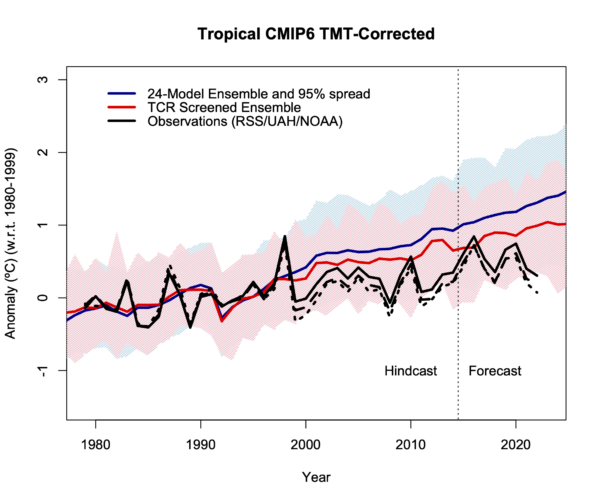
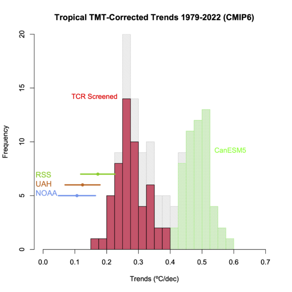
Two things are clear. First the 24-model ensemble as a whole is clearly warming faster than the observations, but the histogram shows that this ensemble is heavily skewed by including 53 ensemble members from CanESM5/CanESM5-CanOE (green in the histogram) which unfortunately has a very high climate sensitivity (ECS 5.6ºC, TCR 2.7ºC). The TCR Screened ensemble (only including the 15 models that have 1.4ºC < TCR < 2.2ºC) is in red and is closer to the observations in terms of trends, but only 7 simulations (from 6 models) out of 53 simulations have trends within the uncertainties of the observations.
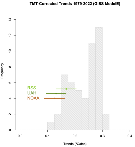
The above selection of CMIP6 models does not include the range of configurations of the GISS coupled models that we looked at in Casas et al. (2023). Since this is a somewhat differently designed ensemble, I’ll plot that similarly (45 simulations), and note too that these are global means, again, for the corrected-TMT product (for the historical and SSP2-45 scenarios after 2014). This ensemble samples model structural variability (vertical resolution, model top, interactive composition) and some aspects of forcing uncertainty (notably for aerosols and ozone), as well as the initial-condition (‘weather’) variability we are used to seeing.
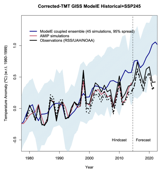
As above, the GISS ensemble diverges slightly from the observations. I’ve also included a line for the AMIP ensemble mean (red) (simulations that use the observed sea surface temperatures as an additional forcing) which shows that the specifics of the interannual variability and observed trend can be matched if the sequence of El Niño and La Niña etc. are matched. For the 1979-2022 trends, the GISS ensemble is a closer match to the observations then the 24-model selection shown above – particularly the GISS-E2.2 simulations all of which are within the uncertainties of the observational spread.
The point of this exercise is first, to include CMIP6 in the comparisons. While we know that this is a trickier ensemble to work with because of the broad (and unrealistic) spread in climate sensitivity, the point in highlighting the GISS model efforts here too is to point out that we are starting to do a better job in terms of sampling different kinds of uncertainty. The CMIP ensembles are still ‘ensembles of opportunity’, but increasingly we are able to take slices through the ensemble to isolate different kinds of sensitivity that are perhaps orthogonal to what has been possible before and make a difference to many observational comparisons – not just the MSU records.
Update (3/19):
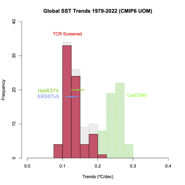
Since I’m making new graphs, here are the SST comparisons as well. The SST files come from the U. Melbourne collation and have 135 simulations from 13 separate models (when I downloaded them) (for the historical runs continued by SSP2-45). Unfortunately, a large part of the ensemble is again the CanESM5 model (52 runs), but there are 73 simulations from 9 models that pass the TCR screen used above. I’m plotting the HadSST4 and ERSSTv5 global means for the observations. The ensemble subsets don’t quite overlap (there are two additional models here – CIESN and GISS-E2.1-G, 14 missing ones, and 11 in common), but the overall picture is very similar. There is a subset of models with high TCR/ECS that warm too quickly, but the bulk of the remaining models are doing well.
The SST comparisons have popped up on twitter in the last few months, led by Roy Spencer who didn’t point out the obvious bifurcation in models, and then repeated by a number of wannabe contrarians who don’t know what they are posting and care even less. Maybe these graphs will be useful for adding some clarity?
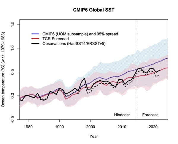
The contrast between the excellent agreement of the screened ensemble for global SST and the slight overestimate (on average) for the tropical or global corrected-TMT is interesting. A couple of things will likely play into that. First the MSU TMT diagnostics are more dominated by changes in the tropics than the surface fields because of the effects of convection, and so the exceptional nature of the La Niña-like trend in the Eastern Pacific Lee et al (2021) is going to be magnified aloft. Second, the impact of forcings is slightly different at different layers, notably for aerosols and ozone changes, and so uncertainties there may be playing different roles in different levels.
One final caveat, I’ve been rather lazy in plotting these ensembles so that I can show the impact of both forced changes and the spread due to internal variability and structural uncertainty. Unfortunately, when you have an ensemble that has fifty runs from a single model and then a handful of models with only one or two runs, then it’s hard to know what’s best. Some papers have taken a single run from each model which seems fair, but actually confuses structural uncertainty and internal variability. Some take the ensemble mean of each model and then plots the average of the averages, which might be a good estimate of the forced change, but loses the information from the weather. Maybe these things need to be estimated separately and put together artificially. Another post though…
References
- S. Po-Chedley, J.T. Fasullo, N. Siler, Z.M. Labe, E.A. Barnes, C.J.W. Bonfils, and B.D. Santer, "Internal variability and forcing influence model–satellite differences in the rate of tropical tropospheric warming", Proceedings of the National Academy of Sciences, vol. 119, 2022. http://dx.doi.org/10.1073/pnas.2209431119
- Q. Fu, C.M. Johanson, S.G. Warren, and D.J. Seidel, "Contribution of stratospheric cooling to satellite-inferred tropospheric temperature trends", Nature, vol. 429, pp. 55-58, 2004. http://dx.doi.org/10.1038/nature02524
- Z. Hausfather, K. Marvel, G.A. Schmidt, J.W. Nielsen-Gammon, and M. Zelinka, "Climate simulations: recognize the ‘hot model’ problem", Nature, vol. 605, pp. 26-29, 2022. http://dx.doi.org/10.1038/d41586-022-01192-2
- M.C. Casas, G.A. Schmidt, R.L. Miller, C. Orbe, K. Tsigaridis, L.S. Nazarenko, S.E. Bauer, and D.T. Shindell, "Understanding Model‐Observation Discrepancies in Satellite Retrievals of Atmospheric Temperature Using GISS ModelE", Journal of Geophysical Research: Atmospheres, vol. 128, 2022. http://dx.doi.org/10.1029/2022JD037523
- S. Lee, M. L’Heureux, A.T. Wittenberg, R. Seager, P.A. O’Gorman, and N.C. Johnson, "On the future zonal contrasts of equatorial Pacific climate: Perspectives from Observations, Simulations, and Theories", npj Climate and Atmospheric Science, vol. 5, 2022. http://dx.doi.org/10.1038/s41612-022-00301-2
I wonder what difference it would make to include primary energy consumption (PEC). We use about 600 exajoules of PEC, corresponding to a forcing of 0.037W/m2 on a global sclae. By all accounts that is a small forcing, and a fraction of it even comes from solar energy eventually. However, similar small forcings have been taken into account, but not this one.
More importantly PEC is concentrated in certain regions. PEC in Germany for instance amounts to 1.09W/m2, not a negligible figure. In the more poplulated third of China it is even 1.5W/m2.
The problem is, this forcing is highly significant in the industrious regions of the planet. There it may well mask other assumed causes of causes of “global” warming, despite being a regional issue. There and then the models may produce an erroneous “good fit”..
I appreciate any refinement in the data. However, for those of us concerned with global warming the Keeling Curve is an essential marker. Methane emissions, while much harder to fully track sit on top of the CO2 data and show evidence that its moving in the direction of exponential upward change and merits deep concern. Arctic amplification may also pose great concern for the average person.
What’s up with the pale gray text? The main text in the article is coming up at 80% of the brightness of whitest white, and the text I see while typing this comment is even whiter.
Update: After I left the above comment, the gray text became much less white, but it still seems to be an example of the recent fad of making regular text gray instead of black.
When I access RealClimate on my old flip phone, I can’t read the pages or the comments at all. Completely invisible. I wish they’d go to black print.
A likely factor in observed TMT is the apparently ongoing negative ENSO trend since 1979. From some brief tests East Pacific SST trends now appear to be comfortably outside the envelope of all CMIP5 model runs. Either this is a spectacularly low probability period of natural variability or the models are missing/getting wrong some important dynamics.
I recall Mike Mann writing years ago arguing that paleo data pointed to a tendency for strong forced warming to cause a La Nina-like SST pattern. Have there been many developments on that idea?
@Paul S says: – ” the models are missing/getting wrong some important dynamics. ”
ms: — La Nina years can be ~0.5°C cooler as they push & hide large amounts of energy into the western Pacific, while El Nino years release more energy stored in the Pacific Ocean.
The Earth Energy Imbalance @ Top Of Atmosphere (EEI @ TOA) was close to zero W/m² (neither warming nor cooling) in 2010, also a very hot El Nino year, while in 2011-12, a strong El Nina year, the EEI was increased again to almost 1.5W/m². El Nino years thus moderate the increase in global warming and are therefore more advantageous for the earth’s climate in the long term.
This is IMO due to the generally higher relative humidity and cloud cover of El Ninos. In the graph of the Met Office for RH you can recognize the El Nino years 1998, 2010, 2016 by the maximum peaks.
https://climate.metoffice.cloud/dashfigs/humidity_RH.png
https://pub.mdpi-res.com/atmosphere/atmosphere-12-01297/article_deploy/html/images/atmosphere-12-01297-g004.png?1634310863
My suspicion is that evaporation, relative humidity and cloud cover are not represented dynamically enough in most models. Note that the Clausius-Clapeyron equation is only valid in closed energy systems and our atmosphere is an open system.
Doktor
Clausius Clappeyrons principle follows from your cooling effect of evapotranspiration kept in combination with the permanence of matter and the permanence of energy in open systems,…..
……… and not by the permanence of die Deutsche Demokratische Rerpublik and its Anerkennung as you have been brought up to it in that closed system,……
……… where the Matter and its energies is dia- lectic, created, mooved and annihilated again by the Godfather, the anonymeous Party Secretary deputee.
I repeat…….
@crabonito
— Are you crazy …my friend ???
Gehst du in die Anstalt – ! ohne LSD !
@craponito
The Clausius–Clapeyron relation characterizes behavior of a closed system during a phase change at constant temperature and pressure. — https://en.wikipedia.org/wiki/Closed_system
He is telling us that a wet towel in air will not dry up faster when heated up, and a pool of water will not freeze faster when the weather cools down.. Because both are no closed systems.
In that way, the fameous Arbeiter and Bauern- faculty of the late peoples republic can reject any critical remark to their propaganda..
Dia Lectic Materialism has allways the upper hand on what is what and what is not and what is appliciable to what or not.
His peculiar style of thought betrays his learnings bacground all the way.
I often find . the fanatic blatant surrealists in the climate dispute in that peculiar class-
It hardly surprizes me anymore.
They are simply lacking legally absolved Mittlere reife, Bachelor 1 because they visited the grand old partys new and progressive political KADRE or “leading class” substitute for it instead.. .
NOAA STARv5 uses the formula TTT = 1.15*TMT – 0.15*TLS and gets +0.142 C/decade from 1979/01 to 2023/02. Using the same formula on UAHv6 we get +0.147 C/decade. RSSv4 provides TTT directly and gets +0.167 C/decade.
STARv5 provides a TLT product from 1981/01 to 2023/02 which shows +0.129 C/decade as compared to UAHv6 of +0.139 C/decade and RSSv4 of +0.219 C/decade.
UAH uses the formula TLT = 1.538*TMT – 0.548*TUT + 0.10*TLS and gets +0.139 C/decade. Using the same formula on STARv5 we get +0.135 C/decade. There is a small discrepancy between the STARv5 official TLT trend +0.129 C/decade and the calculated trend of +0.135 C/decade using the Spencer et al. 2017 method. This is all for the period 1981/01 to 2023/02 since STAR only provides TUT starting in 1981.
Does anyone know why STARv5 uses the :Spencer et al. 2017 method for their TLT product?
Zou et al. 2023 – DOI: 10.1029/2022JD037472
Spencer et al. 2017 – DOI: 10.1007/s13143-017-0010-y
This is all so real and people walk around saying that they want change for the climate bit they do nothing, just talk. SoI took the time to call for a real revolution and wrote a song about negligence when it comes to climate change. So many people protest but still buy the newest cell phones, clothes and splurge. It is time for them to really make a stand, start a real revolution and fight for those making cents an hour just to feed their families.
In case you all wanna share here is a link to the music video: https://www.youtube.com/watch?v=eYfNaKx4g5U&list=PLpuc4AxAeGBHmauqqkIcj90VpU6Q9YHOf&index=1
Thank you all and lets stand together for real change,
Areeyedee
Wouldn’t it make sense to use all the data but use weights so that each of multiple runs from the same model have low weight compared to one run from a different model?
Did any of the climate models predict that this would be the case with the climate this spring?
ICE AND SNOW TO EXTEND INTO APRIL
The month of March has been an exceptionally cold and snowy month. And looking ahead, active patterns with abundant snows and historic lows are forecast to continue into April .
March in the town of Jackson, Wyoming–for example–will end up with temperatures roughly 10F below the long-term average, making the month reminiscent of a typical February.
This has also been a very cold and long-duration winter as a whole for Jackson. It hasn’t seen 50F since Nov 2, a streak of 147 days, which is approaching, and has a chance of besting, the longest streak on record — 163 days.
Coming up, additional heavy snow is forecast across the mid to higher elevations of the Tetons.
Even valleys should expect accumulations — rare for April.
Cold will accompany the snow, and will engulf a larger portion of the CONUS–and also Canada.
Winter is refusing to let-up
https://electroverse.info/records-slain-across-midwest-snowy-california-ice-and-snow-to-extend-into-april-israels-cold-spring-new-zealand/
JS: Did any of the climate models predict that this would be the case with the climate this spring?
BPL: Probably not. Why would you expect them to? They are climate models, not weather models.
How is this temperature record that is 110 years old shown on the climate models in your world that is about to be incinerated due to carbon dioxide?
World Meteorological Organization Assessment of the Purported World Record 58°C Temperature Extreme at El Azizia, Libya (13 September 1922)
“On 13 September 1922, a temperature of 58°C (136.4°F) was purportedly recorded at El Azizia (approximately 40 kilometers south-southwest of Tripoli) in what is now modern-day Libya…………. The WMO assessment is that the highest recorded surface temperature of 56.7°C (134°F) was measured on 10 July 1913 at Greenland Ranch (Death Valley) CA USA.”
http://journals.ametsoc.org/doi/abs/10.1175/BAMS-D-12-00093.1?af=R&
John, the difference between climate and weather is again one of the many things of which you lack the most basic grasp.
Ray Ladbury says on 3 APR 2023 AT 10:59 AM
John, the difference between climate and weather is again one of the many things of which you lack the most basic grasp. Ray Ladbury needs to grasp onto this and explain if these records are the difference between climate and weather.
There is no need to know any of the thing that you so desperately lack and that is ‘science’ to being able to understand what valid historical information is telling us, that it has been 110 years since this all-time high record temperature has been broken and that is that all your hoax about anthropogenic climate change rest on is increasing temperatures on earth, which is not happening as the records show.
This is a record that still holds after 110 years & isn’t it the same WMO that said that this is the warmest time in earth’s history, or some other such nonsense?
http://journals.ametsoc.org/doi/abs/10.1175/BAMS-D-12-00093.1?af=R&
Notice the date that this occurred one hundred years ago.
The town of Marble Bar in Western Australia is legendary for its hot weather. From Oct. 31, 1923, to April 7, 1924, the tiny town scorched with 160 consecutive days over 100 degrees Fahrenheit (37.8 degrees Celsius). That’s a world record.
Think of the 194 people in Marble Bar next time it gets hot in your hometown. Their average high temperature is over 100 F for January, February, March, November and December (the summer months in the Southern Hemisphere).
https://www.livescience.com/30198-weird-weather-anomalies-110302.html
JS: it has been 110 years since this all-time high record temperature has been broken and that is that all your hoax about anthropogenic climate change rest on is increasing temperatures on earth, which is not happening as the records show.
BPL: Warming isn’t counted by “when the hottest record was broken anywhere.” It’s calculated using a trend involving 1) ALL 2) the WORLD’S data points. Not the record in one place once.
Take a statistics course, John. You’re embarrassing yourself.
Sadly, John isn’t embarrassing himself, as he apparently lacks the requisite self-awareness. He’s embarrassing others on his behalf, though.
The wonderful thing from a denier’s POV about all time records is that you get to throw away every bit of data except a single data point. All the other thousands upon thousands of data points get ignored.
Of course, as you surely know, there ARE ways to use all time records to test if there is a trend. You do this by looking at the rates and ratios of new all time highs to new all time lows at a large number of locations. Actuaries have developed more refined tests as well since insurers would go broke fast if they could not model extreme events and their trends. But of course our resident deniers ignore actual real world experts in such things..
This has been done in many studies and the warming trend is quite easily seen there too.
Lastly, this is merely a fairly sad variant of the old tobacco denial saw that Gramps lived to 102 and smoked every day “therefore” tobacco doesn’t cause cancer. Stupid then and just as stupid now as any sort of statistical proof of anything whatsoever. Yet he said it.
Freeman Dyson had this to say a while back:
‘”… I have studied the climate models and I know what they can do. The models solve the equations of fluid dynamics, and they do a very good job of describing the fluid motions of the atmosphere and the oceans. They do a very poor job of describing the clouds, the dust, the chemistry and the biology of fields and farms and forests. They do not begin to describe the real world that we live in. The real world is muddy and messy and full of things that we do not yet understand. It is much easier for a scientist to sit in an air-conditioned building and run computer models, than to put on winter clothes and measure what is really happening outside in the swamps and the clouds. That is why the climate model experts end up believing their own models.”
http://www.edge.org/documents/archive/edge219.html#dysonf
Page not found
The requested page “/documents/archive/edge219.html” could not be found.
Freeman Dyson, aka Not-A-Climate-Scientist, was a brilliant physicist. No doubt there. However, he did not understand climate models, nor did he understand the role they play in climate science. The validity of anthropogenic greenhouse warming is in no way predicated on the correctness of the minute details of the models.
It is warming. That is a simple fact.
It has warmed nearly a degree C on a ~40% increase in CO2. Again, a simple fact.
There are likely feedbacks in the climate system that mean additional warming is still in the pipeline–a high probability.
So, given the FACT that anthropogenic warming is occurring, if the models are crap, then we are in the position of a pilot trying to land in the fog with faulty instruments. Indeed, the models are one of the most significant constraints supporting the lower end of climate sensitivity. If the models were crap, that would strongly argue for extreme caution, not reckless abandon.
Fortunately, however, the models actually do a pretty damn good job for what we need them to do.
Dyson didn’t want climate change to be real because it would have gotten in the way of his Star Trek fantasy future. Argument from consequences–even smart people succumb to logical fallacies when the facts threaten their golden ox.
With the new “STAR” Dataset the average of the trend slopes of the available datasets ( also UAH and RSS) is 0.136 K/ dec. and the best estimate of trend slopes (“TCR adjusted to a best estimate of 1.8K/2*CO2) of the CMIP6’s is 0.26 K/dec. which is 91% more than observed. All these calculations are deduced from tropical TMT from 1979 ( 1981 for STAR) to 2022, following Gavins figure.
In the Update Gavin shows for the SST (part of the GMST) there is not such a difference beween CMIP6’s and observations.
For me it seems to be, that the models run significantly too hot in the tropical TMT but not so on the ground. Any explanation? The origin of modelled “tropical hotspot” ( which is not such a hot hotspot following satellite based observations) is AFAIK the water vapour feedback which seems to be smaller than the CMIP6’s estimate. However, this would also have an impackt on the modelling of the GMST?? Any plausible proposals?
This is just a guess but this study appears relevant
Causes of Higher Climate Sensitivity in CMIP6 Models
https://agupubs.onlinelibrary.wiley.com/doi/full/10.1029/2019GL085782
Where do the outlier TCR results fit in, discussed here https://e360.yale.edu/features/why-clouds-are-the-key-to-new-troubling-projections-on-warming
@chris says: – ” why-clouds-are-the-key…”
ms: — I would like to expressly warn you against considering the ongoing loss of cloud albedo solely as feedback on increasing CO2 concentrations. The ongoing loss of evaporative landscapes (e.g. desertification, dry regions get drier, UHI,…) are obviously a much better explanation for this trend.
It is just as undeniable as the increase in greenhouse gases and is directly linked to human-caused land-use changes incl. hydrological cycles over land. A declining relative humidity observed for decades can help us to quantify these losses of evaporation and clouds. (see my website)
I think some of the statements in the link you sent are simply wrong – e.g.:
– ” Generally, at a global level, models have suggested that the warming and cooling effects cancel each other out,…”
ms: — The difference in SW-down-surface between “all sky” and “clear sky” is at least ~ +54W/m² and a complete loss of the clouds alone would increase the earth’s temperature by ~ 4 – 5°C. However, a clear sky also reduce the GHE by ~ -28W/m² and SW absorbed by atmosphere by ~ -7W/m²
https://climateprotectionhardware.files.wordpress.com/2023/03/cre-cloud-2.png
CERES data from the last 2 decades combined with climate models from the turn of the millennium leave no doubt about this.
https://climateprotectionhardware.files.wordpress.com/2023/03/geb_2000-2020finish.png?w=1024
So I put the ECS for a doubling of CO2 at ~ +1.5°C, much lower than most climate science does.
That’s 3 years old. What’s the research indicating since?