Every so often people who are determined to prove a particular point will come up with a new way to demonstrate it. This new methodology can initially seem compelling, but if the conclusion is at odds with other more standard ways of looking at the same question, further investigation can often reveal some hidden dependencies or non-robustness. And so it is with the new graph being cited purporting to show that the models are an “abject” failure.
Climate modelling
State of Antarctica: red or blue?
A couple of us (Eric and Mike) are co-authors on a paper coming out in Nature this week (Jan. 22, 09). We have already seen misleading interpretations of our results in the popular press and the blogosphere, and so we thought we would nip such speculation in the bud.
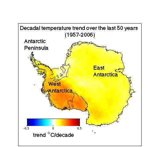
The paper shows that Antarctica has been warming for the last 50 years, and that it has been warming especially in West Antarctica (see the figure). The results are based on a statistical blending of satellite data and temperature data from weather stations. The results don’t depend on the statistics alone. They are backed up by independent data from automatic weather stations, as shown in our paper as well as in updated work by Bromwich, Monaghan and others (see their AGU abstract, here), whose earlier work in JGR was taken as contradicting ours. There is also a paper in press in Climate Dynamics (Goosse et al.) that uses a GCM with data assimilation (and without the satellite data we use) and gets the same result. Furthermore, speculation that our results somehow simply reflect changes in the near-surface inversion is ruled out by completely independent results showing that significant warming in West Antarctica extends well into the troposphere. And finally, our results have already been validated by borehole thermometery — a completely independent method — at at least one site in West Antarctica (Barrett et al. report the same rate of warming as we do, but going back to 1930 rather than 1957; see the paper in press in GRL).
FAQ on climate models: Part II
This is a continuation of a previous post including interesting questions from the comments.
More Questions
- What are parameterisations?
Some physics in the real world, that is necessary for a climate model to work, is only known empirically. Or perhaps the theory only really applies at scales much smaller than the model grid size. This physics needs to be ‘parameterised’ i.e. a formulation is used that captures the phenomenology of the process and its sensitivity to change but without going into all of the very small scale details. These parameterisations are approximations to the phenomena that we wish to model, but which work at the scales the models actually resolve. A simple example is the radiation code – instead of using a line-by-line code which would resolve the absorption at over 10,000 individual wavelengths, a GCM generally uses a broad-band approximation (with 30 to 50 bands) which gives very close to the same results as a full calculation. Another example is the formula for the evaporation from the ocean as a function of the large-scale humidity, temperature and wind-speed. This is really a highly turbulent phenomena, but there are good approximations that give the net evaporation as a function of the large scale (‘bulk’) conditions. In some parameterisations, the functional form is reasonably well known, but the values of specific coefficients might not be. In these cases, the parameterisations are ‘tuned’ to reproduce the observed processes as much as possible.
FAQ on climate models
We discuss climate models a lot, and from the comments here and in other forums it’s clear that there remains a great deal of confusion about what climate models do and how their results should be interpreted. This post is designed to be a FAQ for climate model questions – of which a few are already given. If you have comments or other questions, ask them as concisely as possible in the comment section and if they are of enough interest, we’ll add them to the post so that we can have a resource for future discussions. (We would ask that you please focus on real questions that have real answers and, as always, avoid rhetorical excesses).
Part II is here.
Tropical tropospheric trends again (again)
Many readers will remember our critique of a paper by Douglass et al on tropical tropospheric temperature trends late last year, and the discussion of the ongoing revisions to the observational datasets. Some will recall that the Douglass et al paper was trumpeted around the blogosphere as the definitive proof that models had it all wrong.
At the time, our criticism was itself criticised because our counterpoints had not been submitted to a peer-reviewed journal. However, this was a little unfair (and possibly a little disingenuous) because a group of us had in fact submitted a much better argued paper making the same principal points. Of course, the peer-review process takes much longer than writing a blog post and so it has taken until today to appear on the journal website.
[Read more…] about Tropical tropospheric trends again (again)
Climate change methadone?
Geoengineering is increasingly being discussed (not so sotto voce any more) in many forums. The current wave of interest has been piqued by Paul Crutzen’s 2005 editorial and a number of workshops (commentary) and high profile advocacy. But most of the discussion has occurred in almost total ignorance of the consequences of embarking on such a course.
A wider range of people have now started to publish relevant studies – showing clearly the value of continued research on the topic – and a key one came out this week in JGR-Atmospheres. Robock et al used a coupled GCM with interactive aerosols to see what would happen if they injected huge amounts of SO2 (the precursor of sulphate aerosols) into the tropical or Arctic stratosphere. This is the most talked about (and most feasible) geoengineering idea, based on the cooling impacts of large tropical volcanic eruptions (like Mt. Pinatubo in 1991). Bottom line? This is no panacea.
[Read more…] about Climate change methadone?
More PR related confusion
It’s a familiar story: An interesting paper gets published, there is a careless throwaway line in the press release, and a whole series of misleading headlines ensues.
This week, it’s a paper on bromine- and iodine-mediated ozone loss in marine boundary layer environments (see a good commentary here). This is important for the light that it shines on tropospheric ozone chemistry (“bad ozone”) which is a contributing factor to global warming (albeit one which is about only about 20% as important as CO2). So far so good. The paper contains some calculations indicating that chemical transport models without these halogen effects overestimate ozone near the Cape Verde region by about 15% – a difference that certainly could be of some importance if it can be extrapolated across the oceans.
However, the press release contains the line
Large amounts of ozone – around 50% more than predicted by the world’s state-of-the-art climate models – are being destroyed in the lower atmosphere over the tropical Atlantic Ocean.
(my highlights). Which led directly to the headlines like Study highlights need to adjust climate models.
Why is this confusing? Because the term ‘climate models’ is interpreted very differently in the public sphere than it is in the field. For most of the public, it is ‘climate models’ that are used to project global warming into the future, or to estimate the planet’s sensitivity to CO2. Thus a statement like the one above, and the headline that came from it are interpreted to mean that the estimates of sensitivity or of future warming are now in question. Yet this is completely misleading since neither climate sensitivity nor CO2 driven future warming will be at all affected by any revisions in ozone chemistry – mainly for the reason that most climate models don’t consider ozone chemistry at all. Precisely zero of the IPCC AR4 model simulations (discussed here for instance) used an interactive ozone module in doing the projections into the future.
What the paper is discussing, and what was glossed over in the release, is that it is the next generation of models, often called “Earth System Models” (ESMs), that are starting to include atmospheric chemistry, aerosols, ozone and the like. These models may well be significantly affected by increases in marine boundary layer ozone loss, but since they have only just started to be used to simulate 20th and early 21st Century changes, it is very unclear what difference it will make at the large scale. These models are significantly more complicated than standard climate models (having dozens of extra tracers to move around, and a lot of extra coding to work through), are slower to run, and have been used much less extensively.
Climate models today are extremely flexible and configurable tools that can include all these Earth System modules (including those mentioned above, but also full carbon cycles and dynamic vegetation), but depending on the application, often don’t need to. Thus while in theory, a revision in ozone chemistry, or soil respiration or aerosol properties might impact the full ESM, it won’t affect the more basic stuff (like the sensitivity to CO2). But it seems that the “climate models will have to be adjusted” meme is just too good not to use – regardless of the context.
Ocean heat content revisions
Hot on the heels of last months reporting of a discrepancy in the ocean surface temperatures, a new paper in Nature (by Domingues et al, 2008) reports on the revisions of the ocean heat content (OHC) data – a correction required because of other discrepancies in measuring systems found last year.
Tropical tropospheric trends again
Back in December 2007, we quite heavily criticised the paper of Douglass et al (in press at IJoC) which purported to show that models and data were inconsistent when it came to the trends in the tropical troposphere. There were two strands to our critique: i) that the statistical test they used was not appropriate and ii) that they did not acknowledge the true structural uncertainty in the observations. Most subsequent discussion has been related to the statistical issue, but the second point is perhaps more important.
Even when Douglass et al was written, those authors were aware that there were serious biases in the radiosonde data (they had been reported in Sherwood et al, 2005 and elsewhere), and that there were multiple attempts to objectively address the problems and to come up with more homogeneous analyses. We mentioned the RAOBCORE project at the time and noted the big difference using their version 1.4 vs 1.2 made to the comparison (a difference nowhere mentioned in Douglass et al’s original accepted paper which only reported on v1.2 despite them being aware of the issue). However, there are at least three new papers in press that independently tackle the issue, and their results go a long towards addressing the problems.
[Read more…] about Tropical tropospheric trends again
How to cook a graph in three easy lessons
These days, when global warming inactivists need to trot out somebody with some semblance of scientific credentials (from the dwindling supply who have made themselves available for such purposes), it seems that they increasingly turn to Roy Spencer, a Principal Research Scientist at the University of Alabama. Roy does have a handful of peer-reviewed publications, some of which have quite decent and interesting results in them. However, the thing you have to understand is that what he gets through peer-review is far less threatening to the mainstream picture of anthropogenic global warming than you’d think from the spin he puts on it in press releases, presentations and the blogosphere. His recent guest article on Pielke Sr’s site is a case in point, and provides the fodder for our discussion today.
[Read more…] about How to cook a graph in three easy lessons