This month’s open thread. Northern Hemisphere Spring is on it’s way, along with peak Arctic/minimum Antarctic sea ice, undoubtedly more discussion about the polar vortex, and the sharpening up of the (currently very uncertain) ENSO forecast for the rest of this year.
Search Results for: SST
Update day 2021
As is now traditional, every year around this time we update the model-observation comparison page with an additional annual observational point, and upgrade any observational products to their latest versions.
A couple of notable issues this year. HadCRUT has now been updated to version 5 which includes polar infilling, making the Cowtan and Way dataset (which was designed to address that issue in HadCRUT4) a little superfluous. Going forward it is unlikely to be maintained so, in a couple of figures, I have replaced it with the new HadCRUT5. The GISTEMP version is now v4.
For the comparison with the Hansen et al. (1988), we only had the projected output up to 2019 (taken from fig 3a in the original paper). However, it turns out that fuller results were archived at NCAR, and now they have been added to our data file (and yes, I realise this is ironic). This extends Scenario B to 2030 and Scenario A to 2060.
Nothing substantive has changed with respect to the satellite data products, so the only change is the addition of 2020 in the figures and trends.
So what do we see? The early Hansen models have done very well considering the uncertainty in total forcings (as we’ve discussed (Hausfather et al., 2019)). The CMIP3 models estimates of SAT forecast from ~2000 continue to be astoundingly on point. This must be due (in part) to luck since the spread in forcings and sensitivity in the GCMs is somewhat ad hoc (given that the CMIP simulations are ensembles of opportunity), but is nonetheless impressive.
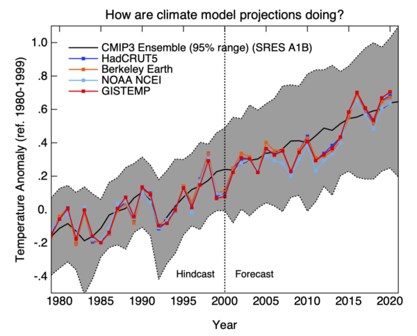
The forcings spread in CMIP5 was more constrained, but had some small systematic biases as we’ve discussed Schmidt et al., 2014. The systematic issue associated with the forcings and more general issue of the target diagnostic (whether we use SAT or a blended SST/SAT product from the models), give rise to small effects (roughly 0.1ºC and 0.05ºC respectively) but are independent and additive.
The discrepancies between the CMIP5 ensemble and the lower atmospheric MSU/AMSU products are still noticeable, but remember that we still do not have a ‘forcings-adjusted’ estimate of the CMIP5 simulations for TMT, though work with the CMIP6 models and forcings to address this is ongoing. Nonetheless, the observed TMT trends are very much on the low side of what the models projected, even while stratospheric and surface trends are much closer to the ensemble mean. There is still more to be done here. Stay tuned!
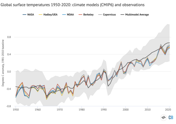
The results from CMIP6 (which are still being rolled out) are too recent to be usefully added to this assessment of forecasts right now, though some compilations have now appeared:
The issues in CMIP6 related to the excessive spread in climate sensitivity will need to be looked at in more detail moving forward. In my opinion ‘official’ projections will need to weight the models to screen out those ECS values outside of the constrained range. We’ll see if other’s agree when the IPCC report is released later this year.
Please let us know in the comments if you have suggestions for improvements to these figures/analyses, or suggestions for additions.
References
- Z. Hausfather, H.F. Drake, T. Abbott, and G.A. Schmidt, "Evaluating the Performance of Past Climate Model Projections", Geophysical Research Letters, vol. 47, 2020. http://dx.doi.org/10.1029/2019GL085378
- G.A. Schmidt, D.T. Shindell, and K. Tsigaridis, "Reconciling warming trends", Nature Geoscience, vol. 7, pp. 158-160, 2014. http://dx.doi.org/10.1038/ngeo2105
2020 Hindsight
Yesterday was the day that NASA, NOAA, the Hadley Centre and Berkeley Earth delivered their final assessments for temperatures in Dec 2020, and thus their annual summaries. The headline results have received a fair bit of attention in the media (NYT, WaPo, BBC, The Guardian etc.) and the conclusion that 2020 was pretty much tied with 2016 for the warmest year in the instrumental record is robust.
[Read more…] about 2020 HindsightThe number of tropical cyclones in the North Atlantic
2020 has been an unusual and challenging year in many ways. One was the record-breaking number of named tropical cyclones in the North Atlantic (and the Carribean Sea). There has been 30 named North Atlantic tropical cyclones in 2020, beating the previous record of 28 from 2005 by two.
A natural question then is whether we can expect this high number in the future or if the number of tropical storms will continue to increase. A high number of such events is equivalent to a high frequency of tropical cyclones.
But we should expect fewer tropical cyclones generally in a warmer world according to the IPCC “SREX” report from 2012, and those that form may become even more powerful than the ones that we have observed to date:
There is generally low confidence in projections of changes in extreme winds because of the relatively few studies of projected extreme winds, and shortcomings in the simulation of these events. An exception is mean tropical cyclone maximum wind speed, which is likely to increase, although increases may not occur in all ocean basins. It is likely that the global frequency of tropical cyclones will either decrease or remain essentially unchanged…
So how does this conclusion relate to the number of tropical cyclones in the North Atlantic with a new record this season? One reason to look in more detail at the North Atlantic is because its observational record is believed to be more complete and more reliable than for other regions around the world.
The observational record may also suggest that the number of tropical cyclones in the North Atlantic has increased slowly over the 50 years in addition to year-to-year fluctuations around this trend (black symbols in Fig 1).
We know that the number of cyclones is sensitive to the time of the year (hence, hurricane seasons), phenomena such as El Niño Southern Oscillation (ENSO) and the Madden Julian Oscillation (MJO), and geography (the ocean basin shape and the latitude). We also know that the sea surface needs to be warmer than 26.5°C for them to form.
The role of sea surface temperature is indeed an important factor, and from physical reasoning, one would think that the number of tropical cyclones depends on the area of warm sea surface  (sea surface temperature exceeding 26.5°C).
One explanation for why the area is a key factor may be that the probability of finding favourable conditions with right ‘seed’ for organised convection (e.g. easterly waves) and no wind shear increases when there is a greater region with sufficient sea surface temperatures.
The area of warm sea surface is mentioned in the IPCC SREX that dismisses the expectation that an increase in the area extent of the region of 26°C sea surface temperature should lead to increases in tropical cyclone frequency. Specifically it says that there is
a growing body of evidence that the minimum SST [sea surface temperature] threshold for tropical cyclogenesis increases at about the same rate as the SST increase due solely to greenhouse gas forcing.
On the other hand, there has also been some indication that the number of tropical cyclones does seem to be proportional to the area to the power of 5:  (Benestad, 2008). When this relationship is extended to recent years, as shown with the green and blue curves in Fig 1, we see an increase that this crude estimate more or less follows the observed number of evens.
Global warming implies a greater area with sea surface exceeding the threshold of 26.5°C for tropical cyclone genesis. Also, the nonlinear dependency to implies few events and little trend as long as is below a critical size. The combination of a nonlinear relationship and a critical threshold area could explain why it is difficult to detect a trend in the historical data.
There is some good news in that is limited by the geometry of the ocean basin. Nevertheless, a potential nonlinear connection between the number of tropical cyclones and is a concern. If this cannot be falsified, then the tropical cyclones represent a more potent danger than anticipated by the IPCC SREX conclusions. So let’s hope that somebody is able to show that the analysis presented in (Benestad, 2008) is wrong.
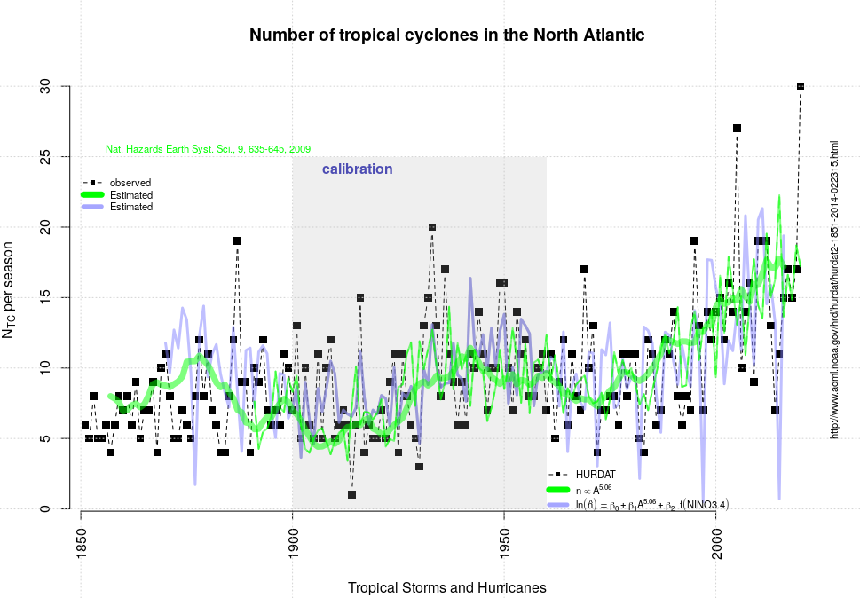
Fig 1. Observed (black symbols) and estimated (green and blue curves) number of named tropical cyclones in the North Atlantic and the Caribbean Sea after (Benestad, 2008). Source: “demo(tropicalcyclones)”.
References
- R.E. Benestad, "On tropical cyclone frequency and the warm pool area", Natural Hazards and Earth System Sciences, vol. 9, pp. 635-645, 2009. http://dx.doi.org/10.5194/nhess-9-635-2009
An ever more perfect dataset?
Do you remember when global warming was small enough for people to care about the details of how climate scientists put together records of global temperature history? Seems like a long time ago…
Nonetheless, it’s worth a quick post to discuss the latest updates in HadCRUT (the data product put together by the UK’s Hadley Centre and the Climatic Research Unit at the University of East Anglia). They have recently released HadCRUT5 (Morice et al., 2020), which marks a big increase in the amount of source data used (similarly now to the upgrades from GHCN3 to GHCN4 used by NASA GISS and NOAA NCEI, and comparable to the data sources used by Berkeley Earth). Additionally, they have improved their analysis of the sea surface temperature anomalies (a perennial issue) which leads to an increase in the recent trends. Finally, they have started to produce an infilled data set which uses an extrapolation to fill in data-poor areas (like the Arctic – first analysed by us in 2008…) that were left blank in HadCRUT4 (so similar to GISTEMP, Berkeley Earth and the work by Cowtan and Way). Because the Arctic is warming faster than the global mean, the new procedure corrects a bias that existing in the previous global means (by about 0.16ºC in 2018 using a 1951-1980 baseline). Combined, the new changes give a result that is much closer to the other products:
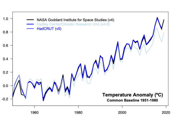
Differences persist around 1940, or in earlier decades, mostly due to the treatment of ocean temperatures in HadSST4 vs. ERSST5.
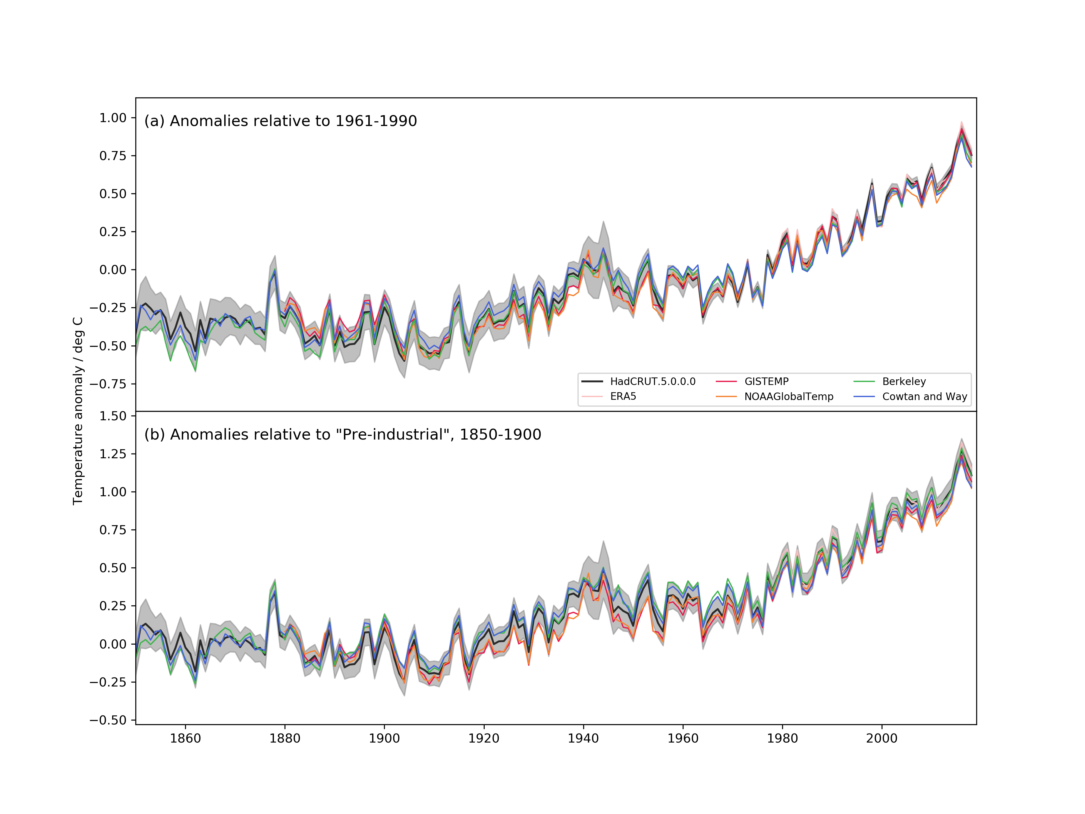
In conclusion, this update further solidifies the robustness of the surface temperature record, though there are still questions to be addressed, and there remain mountains of old paper records to be digitized.
The implications of these updates for anything important (such as the climate sensitivity or the carbon budget) will however be minor because all sensible analyses would have been using a range of surface temperature products already.
With 2020 drawing to a close, the next annual update and intense comparison of all these records, including the various satellite-derived global products (UAH, RSS, AIRS) will occur in January. Hopefully, HadCRUT5 will be extended beyond 2018 by then.
In writing this post, I noticed that we had written up a detailed post on the last HadCRUT update (in 2012). Oddly enough the issues raised were more or less the same, and the most important conclusion remains true today:
First and foremost is the realisation that data synthesis is a continuous process. Single measurements are generally a one-time deal. Something is measured, and the measurement is recorded. However, comparing multiple measurements requires more work – were the measuring devices calibrated to the same standard? Were there biases in the devices? Did the result get recorded correctly? Over what time and space scales were the measurements representative? These questions are continually being revisited – as new data come in, as old data is digitized, as new issues are explored, and as old issues are reconsidered. Thus for any data synthesis – whether it is for the global mean temperature anomaly, ocean heat content or a paleo-reconstruction – revisions over time are both inevitable and necessary.
References
Climate Sensitivity: A new assessment
Not small enough to ignore, nor big enough to despair.
There is a new review paper on climate sensitivity published today (Sherwood et al., 2020 (preprint) that is the most thorough and coherent picture of what we can infer about the sensitivity of climate to increasing CO2. The paper is exhaustive (and exhausting – coming in at 166 preprint pages!) and concludes that equilibrium climate sensitivity is likely between 2.3 and 4.5 K, and very likely to be between 2.0 and 5.7 K.
[Read more…] about Climate Sensitivity: A new assessmentReferences
- S.C. Sherwood, M.J. Webb, J.D. Annan, K.C. Armour, P.M. Forster, J.C. Hargreaves, G. Hegerl, S.A. Klein, K.D. Marvel, E.J. Rohling, M. Watanabe, T. Andrews, P. Braconnot, C.S. Bretherton, G.L. Foster, Z. Hausfather, A.S. von der Heydt, R. Knutti, T. Mauritsen, J.R. Norris, C. Proistosescu, M. Rugenstein, G.A. Schmidt, K.B. Tokarska, and M.D. Zelinka, "An Assessment of Earth's Climate Sensitivity Using Multiple Lines of Evidence", Reviews of Geophysics, vol. 58, 2020. http://dx.doi.org/10.1029/2019RG000678
One more data point
The climate summaries for 2019 are all now out. None of this will be a surprise to anyone who’s been paying attention, but the results are stark.
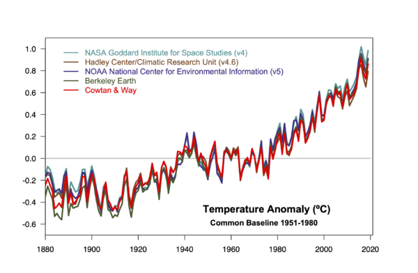
- 2019 was the second warmest year (in analyses from GISTEMP, NOAA NCEI, ERA5, JRA55, Berkeley Earth and Cowtan & Way, RSS TLT), it was third warmest in the standard HadCRUT4 product and in the UAH TLT. It was the warmest year in the AIRS Ts product.
- For ocean heat content, it was the warmest year, though in terms of just the sea surface temperature (HadSST3), it was the third warmest.
- The top 5 years in all surface temperature series, are the last five years. [Update: this isn’t true for the MSU TLT data which have 2010 (RSS) and 1998 (UAH) still in the mix].
- The decade was the first with temperatures more than 1ºC above the late 19th C in almost all products.
This year there are two new additions to the discussion, notably the ERA5 Reanalyses product (1979-2019) which is independent of the surface weather stations, and the AIRS Ts product (2003-2019) which again, is totally independent of the surface data. Remarkably, they line up almost exactly. [Update: the ERA5 system assimilates the SYNOP reports from weather stations, which is not independent of the source data for the surface temperature products. However, the interpolation is based on the model physics and many other sources of observed data.]
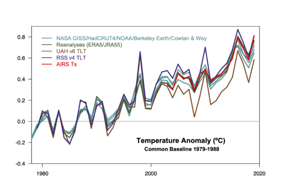
The two MSU lowermost troposphere products are distinct from the surface record (showing notably more warming in the 1998, 2010 El Niño years – though it wasn’t as clear in 2016), but with similar trends. The biggest outlier is (as usual) the UAH record, indicating that the structural uncertainty in the MSU TLT trends remains significant.
One of the most interesting comparisons this year has been the coherence of the AIRS results which come from an IR sensor on board EOS Aqua and which has been producing surface temperature estimates from 2003 onwards. The rate and patterns of warming of this and GISTEMP for the overlap period are remarkably close, and where they differ, suggest potential issues in the weather station network.
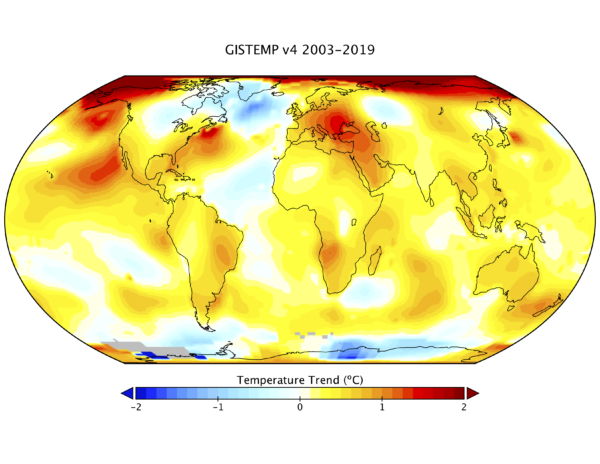
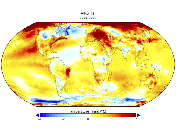
The trends over that period in the global mean are very close (0.24ºC/dec vs. 0.25ºC/dec), with AIRS showing slightly more warming in the Arctic. Interestingly, AIRS 2019 slightly beats 2016 in their ranking.
I will be updating the model/observation comparisons over the next few days.
How much CO2 your country can still emit, in three simple steps
Everyone is talking about emissions budgets – what are they and what do they mean for your country?
Our CO2 emissions are causing global heating. If we want to stop global warming at a given temperature level, we can emit only a limited amount of CO2. That’s our emissions budget. I explained it here at RealClimate a couple of years ago:
First of all – what the heck is an “emissions budget” for CO2? Behind this concept is the fact that the amount of global warming that is reached before temperatures stabilise depends (to good approximation) on the cumulative emissions of CO2, i.e. the grand total that humanity has emitted. That is because any additional amount of CO2 in the atmosphere will remain there for a very long time (to the extent that our emissions this century will like prevent the next Ice Age due to begin 50 000 years from now). That is quite different from many atmospheric pollutants that we are used to, for example smog. When you put filters on dirty power stations, the smog will disappear. When you do this ten years later, you just have to stand the smog for a further ten years before it goes away. Not so with CO2 and global warming. If you keep emitting CO2 for another ten years, CO2 levels in the atmosphere will increase further for another ten years, and then stay higher for centuries to come. Limiting global warming to a given level (like 1.5 °C) will require more and more rapid (and thus costly) emissions reductions with every year of delay, and simply become unattainable at some point.
In her recent speech at the French National Assembly, Greta Thunberg rightly made the emissions budget her central issue.
So let’s look at how the emissions budget concept can be used to guide policy on future emissions trajectories for countries.
[Read more…] about How much CO2 your country can still emit, in three simple stepsUnforced Variations vs Forced Responses?
Guest commentary by Karsten Haustein, U. Oxford, and Peter Jacobs (George Mason University).
One of the perennial issues in climate research is how big a role internal climate variability plays on decadal to longer timescales. A large role would increase the uncertainty on the attribution of recent trends to human causes, while a small role would tighten that attribution. There have been a number of attempts to quantify this over the years, and we have just published a new study (Haustein et al, 2019) in the Journal of Climate addressing this question.
Using a simplified climate model, we find that we can reproduce temperature observations since 1850 and proxy-data since 1500 with high accuracy. Our results suggest that multidecadal ocean oscillations are only a minor contributing factor in the global mean surface temperature evolution (GMST) over that time. The basic results were covered in excellent articles in CarbonBrief and Science Magazine, but this post will try and go a little deeper into what we found.
[Read more…] about Unforced Variations vs Forced Responses?References
- K. Haustein, F.E.L. Otto, V. Venema, P. Jacobs, K. Cowtan, Z. Hausfather, R.G. Way, B. White, A. Subramanian, and A.P. Schurer, "A Limited Role for Unforced Internal Variability in Twentieth-Century Warming", Journal of Climate, vol. 32, pp. 4893-4917, 2019. http://dx.doi.org/10.1175/JCLI-D-18-0555.1
The best case for worst case scenarios
The “end of the world” or “good for you” are the two least likely among the spectrum of potential outcomes.
Stephen Schneider

Scientists have been looking at best, middling and worst case scenarios for anthropogenic climate change for decades. For instance, Stephen Schneider himself took a turn back in 2009. And others have postulated both far more rosy and far more catastrophic possibilities as well (with somewhat variable evidentiary bases).
[Read more…] about The best case for worst case scenariosReferences
- S. Schneider, "The worst-case scenario", Nature, vol. 458, pp. 1104-1105, 2009. http://dx.doi.org/10.1038/4581104a