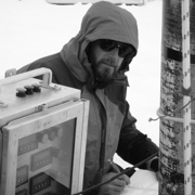
 Eric Steig is an isotope geochemist at the University of Washington in Seattle. His primary research interest is use of ice core records to document climate variability in the past. He also works on the geological history of ice sheets, on ice sheet dynamics, on statistical climate analysis, and on atmospheric chemistry.
He received a BA from Hampshire College at Amherst, MA, and M.S. and PhDs in Geological Sciences at the University of Washington, and was a DOE Global Change Graduate fellow. He was on the research faculty at the University of Colorado and taught at the University of Pennsylvania prior to returning to the University of Washington 2001. He has served on the national steering committees for the Ice Core Working Group, the Paleoenvironmental Arctic Sciences initiative, and the West Antarctic Ice Sheet Initiative, all sponsored by the US National Science Foundation. He was a senior editor of the journal Quaternary Research, and director of the Quaternary Research Center. He has published more than 100 peer-reviewed articles in international journals.
More information about his research and publication record can be found here.
All posts by eric.
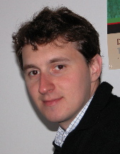
 David Archer is a computational ocean chemist at the University of Chicago. He has published research on the carbon cycle of the ocean and the sea floor, at present, in the past, and in the future. Dr. Archer has worked on the ongoing mystery of the low atmospheric CO2 concentration during glacial time 20,000 years ago, and on the fate of fossil fuel CO2 on geologic time scales in the future, and its impact on future ice age cycles, ocean methane hydrate decomposition, and coral reefs. Archer has written a textbook for non-science major undergraduates called “